R E S E A R C H
Open Access
Scale effect analysis of early-termination
fixed-complexity sphere detector
Rongrong Qian
1, Yuan Qi
2*, Tao Peng
3, Jun Yang
1and Wenbo Wang
3Abstract
In this paper, we show that the early-termination fixed-complexity sphere detector (ET-FSD) has ascale effectwhen being employed in multi-antenna systems that have to detect signals of multiple users under the constraint of sum complexity. The so-called scale effect stands for a kind of effect in which the complexity per user can be reduced as the number of users increases without loss of diversity order. The main contributions of this study are as follows: (1) we establish a mathematical model based on thelarge deviation principleto apply the concept of scale effect to ET-FSD; (2) we prove the existence of the scale effect of ET-FSD in a multi-user scenario; and (3) we demonstrate that within multi-user systems, the scale effect can be exploited to realize ET-FSD that has the optimal performance in the point view of diversity order under polynomial complexity constraint per user.
1 Introduction
1.1 Research on MIMO detection
Consider a spatial-multiplexing input multiple-output (MIMO) system withnT transmit andnR receive antennas, with the channel represented by the matrixH= [h1h2 · · · hnT]∈ CnR×nT, where hi is the ith column of H. All entries of the channel matrix Hare indepen-dent and iindepen-dentically distributed (i.i.d.) zero-mean complex Gaussian random variables with unit variance. Let the entries of the vectors =[s1 s2 · · · snT]T∈ CnT×1be the transmit symbols, with eachsi belonging to the
constel-lation setDwith sizem. The signal model of the MIMO system is given by
y=Hs+v=
nT
i=1
hisi+v,
where yis the received signal vector, and vis the zero-mean circularly symmetric complex Gaussian noise with covariance matrixE(vvH)=σ2InR,nR. We suppose thatH is perfectly known at the receiver. LetEsdenote the energy
at the transmitter per symbol period, i.e.,Es = E(|si|2).
*Correspondence: [email protected]
2Electronic School, Beijing University of Posts and Telecommunications (BUPT), Beijing 100876, China
Full list of author information is available at the end of the article
Without loss of generality, we assume thatEs=1/nTand nR ≥ nT. Under these conditions, the optimal scheme of MIMO detection that minimizes the average error probability is the maximum-likelihood (ML) detector expressed by
sML=arg min
s∈DnTy−Hs
2
F. (1)
In the context of high signal/noise ratio (SNR), the optimality of the ML detector can be interpreted as the full diversity which means that the detector is capable of achieving the diversity order nR [1]. Despite the optimal performance, however, the ML detector is not a promising scheme of MIMO detec-tion in practice because of its extremely high com-plexity. It is evident from (1) that the ML detector has to perform an exhaustive search of mnT possible candidates and, thus, has the exponential complexitya CML=O(mnT).
Ever since MIMO techniques became widely accepted as among the few emerging key technologies for wireless communications, realizing the performance of the opti-mal or near-optiopti-mal MIMO detection without exhaustive search has been an interesting topic for decades [2-9]. It is known from [2-7] that the problem of Equation 1 can be formulated as a lattice search problem [2-4], an integer-least-squares problem [5], a semidefinite relaxation
lem [6], and a shortest path problem [7] which are shown to have their own efficient solution methods (algo-rithms). Many low-complexity strategies can also be used to restrict computational complexity or make the search more efficient, including restricting the search or invoking early termination. Even in recent years, MIMO detection has remained an attractive topic [10-15].
A lot of prior works have been done. However, to the authors’ knowledge, it is still hard to realize the MIMO detector with optimal performance (regarding both error probability and diversity order) with the poly-nomial complexity constraintb. It is shown in [5] that, for integer-least-squares problem with small problem size, the expected complexity of the sphere decoder (SD) at high SNR can be approximated by a polynomial func-tion. The closet-lattice search and shortest path algorithm can efficiently cut down the complexity of solving the integer-least-squares problem [4,7]. However, there does not exist a polynomial upper bound on SD complex-ity [16], closet-lattice search, or shortest path algorithm for any fixed SNR. With some fixed performance degra-dation (14) [16], the SD has an exponential complexity (in both the worst and the average cases) of CSD = O(mγnT) with γ ∈ (0, 1] [16]. The fixed-complexity sphere decoder (FSD) is proved to maintain full diversity with a complexity of CFSD = O(m
√n
T) that is
‘subex-ponential’ [17]. On the other hand, the linear receivers, e.g., zero-forcing (ZF) and minimum mean square error schemes, have low complexity but quite poor diversity order nR− nT +1 [1]. The situation is discouraging as several profound studies show that many MIMO detec-tors have their own inherent limitations [16,18,19]. Under this situation, the authors believe that exploiting more potential positive factors in MIMO detectors might be one of the appropriate ideas to make the next break-through. In this paper, we focus on exploiting the poten-tial positive factor of MIMO detection in a multi-user scenario.
1.2 MIMO detection in a multi-user scenario
It can be found that most studies on the complexity of MIMO detection are under a single-user assumption [2-13], while this study focuses on the complexity of MIMO detection in a multi-user scenario. To understand the motivation behind, one can think of the factor that MIMO receivers in base stations would have to detect signals from multiple-access users. In previous studies [20,21], the scale effect-oriented MIMO detector (SEOD) was developed for multi-user system, which was also shown to have a kind of effect called the scale effect in which the complexity per user can be reduced as the number of users increases without loss of diversity order. Moreover, from [21], we know that scale effect would play an important role in a cloud base station because the cloud
base station is a large-scale multi-user system where the baseband processes of a great number of base stations (each could have a lot of accessed users) are performed together within a virtual base station pool under the limit of overall run-time.
However, a big question left to us is whether the scale effect only exists in SEOD. If the answer is ‘yes’, it will mean that the scale effect has limited practical mean-ings since the SEOD is a very special MIMO detection scheme which has been carefully designed. Whereas if other schemes of MIMO detection also have the scale effect, we would expect that the scale effect could become an important feature of MIMO detection in multi-user scenarios.
1.3 Contributions
In this study, we focus on investigating the early-termination fixed-complexity sphere detector (ET-FSD) that is an extended version of FSD by incorporating early-termination mechanism. The existence of scale effect in ET-FSD is proven (Theorems 2 and 3). Due to the scale effect, the complexity per user of ET-FSD can be kept under a polynomial constraint while maintaining full-diversity performance (Theorem 3). We note that the original FSD has no scale effect; thus, in a multi-user case, it still achieves full diversity with subexponential com-plexity. This result implies that the scale effect not only exists in SEOD but also in ET-FSD and, thus, encourages us to extend and deepen the studies on scale effect in the future. Moreover, an analytical framework based on the large deviation principle is established to investi-gatethe scale effect in this paper, while [20] does not provide such a framework.
1.4 Organization
The rest of this paper is organized as follows: In Section 2, the ET-FSD scheme is specified, and its underlying math-ematical model is presented. In Section 3, we prove that the ET-FSD in a single-user scenario is able to achieve full diversity; meanwhile, the complexity behavior of ET-FSD is studied considering both single-user and multi-user scenarios. With respect to the multi-user scenario, the scale effect of ET-FSD is rigorously defined, which in Section 4 is proven to exist. Consequently, the numerical results are provided in Section 5. We conclude our paper in Section VI.
2 Early-termination fixed-complexity sphere decoder
2.1 ET-FSD scheme
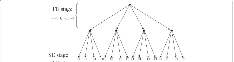
implementation due to its fixed complexity and parallel-computing-friendly features. By simply incorporating an early-termination mechanism into the FSD, we can estab-lish the ET-FSD scheme. The main process of the ET-FSD is a constrained tree search through a tree withnTlevels wherembranches originate from each node. The whole tree search can be realized in two stages: full expansion (FE) and single expansion (SE) search stages, which can be summarized as follows:
• The first stage is the FE search in which a full search is performed inp levels, expanding all m branches per node. In this stage, the transmit symbol with larger noise amplification appears at an earlier level of the tree. Note that a larger noise amplification can also be understood as a smaller post-processing SNR.
• The second stage is the SE search in which a single search needs to be performed in the remaining
nT−plevels. Analogous in principle to previous studies (such as in [17,22]), the SE search expands one branch per node followed by the ZF
estimate.
Besides the constrained tree search, the complete real-ization of the ET-FSD also includes the preprocessing of the channel matrix (as FSD [9,17,22] does), which determines the detection order of the transmit symbols and has two stages as well: the preprocessing for the FE search and that for the SE search. To be specific, the pre-processing of the channel matrix can be expressed by Algorithm 1 using the following notations. (·)† denotes the Moore-Penrose pseudoinverse. FlagET is a flag that determines whether the early termination is enabled in the algorithm or not, i.e., FlagET = True means enabled, otherwise disabled. The function denoted by find(b=x) finds the indices of the elements of the vectorbthat do not equalx. The preprocessing is realized iteratively, and within the jth iteration, the effective channel matrixHj is reconstructed by removing some column from Hj−1, where the initialization condition is H0 = H. Accord-ingly,Pjdenotes the Moore-Penrose pseudoinverse ofHj. Algorithm 1 returnsaas the ordered indices of the trans-mit symbols. The elements of awith indices 1 to pare the indices of the transmit symbols to be detected in the FE search. Then the remaining nT − pelements of aare the indices of the transmit symbols to be detected in the SE search. Furthermore, b =[b1,b2,· · ·,b(nT−j)] is just an intermediate vector with its elements satisfy-ing{b1,b2,· · ·,b(nT−j)} = {1, 2,· · ·,nT} \ {a1,a2,· · ·,aj}. Also, ρ nTEs/σ2 = 1/σ2 is the average SNR at the
receiver (a.k.a. the average receive SNR), andγ ∈(0, 1)is a real value.
Algorithm 1 (a,p) = CHANNELPREPROCESSING(H,p, nT, FlagET,γ)
/ * Initialization * / 1. a:=[0 0 · · · 0]
2. b:=[1 2 · · · nT] 3. j:=0
/ * Preprocessing for FE search stage * / 4. while(j≤p−1)
5. Hj:=[hb1 hb2 · · · hb(nT−j)]
6. Pj:=Hj†
7. imax:=arg max1≤i≤(nT−j)[P
j(Pj)H] i,i 8. a(j+1):=bimax
9. if([Pj(Pj)H]imax,imax≤
1 nTρ
(1−γ )) &&
(FlagET = True)
10. p:=j
11. break
12. end
13. b:=b(find(b=a(j+1))) / * Resetbby
removing a(j+1)from it * /
14. j:=j+1
15. end
/ * Preprocessing for SE search stage * / 16. while(j≤nT−1)
17. a(j+1):=b(j−p+1)
18. end
Compared with the channel preprocessing algorithm of the FSD [9,17,22], Algorithm 1 of the ET-FSD has a newly introduced functionality, as seen in lines 9 to 12, which can terminate early the loop of the preprocessing for the FE search depending on the channel matrix and updatepbefore breaking the loop when FlagET := True is set. Moreover, we havepas one input of Algorithm 1 to guarantee full diversity. Early termination implies that the number of levels of the FE search stage could be less thanp. If we set FlagET := False, Algorithm 1 would exe-cute identically as [17,22]. Thus, FSD could be considered as a special case of ET-FSD. In line 7, the index of the largest diagonal entry of Pj(Pj)H, imax, is found. In fact, the diagonal entries ofPj(Pj)Hreflect the post-processing noise amplification (see (5) as well). In line 8, the origi-nal index of the transmit symbol,a(j+1), is obtained based onimax. It is clear that in thejth iteration of channel pre-processing, thea(j+1)th transmit symbol has the largest noise amplification. In this work, for both the convenience of mathematical analysis and the reduction of computa-tional complexity, ZF is employed in the SE stage. Thus, the preprocessing for the SE stage is performed as in line 17.
channel matrix as the two most significant parameters. Analogous to the FSD, the tree search of the ET-FSD con-sists of two stages and can be illustrated as in Figure 1. On the other hand, we can express such tree search by Algorithm 2, which is in the iterative fashion. Before the details are examined, the required notation can be given as follows: D(k) is the kth element of constel-lation set D; ZF(·,·) denotes the functionality of zero-forcing estimate;sSE[sap+1,sa(p+2), · · ·,sanT]T;HSE
[ha(p+1), ha(p+2), · · ·, hanT];yjis the intermediate vector
in thejth iteration; andsa(j+1) is thea(j+1)th element ofs. The initial input of Algorithm 2 includesy0 := y,j := 0,
dmax := +∞ands :=[0, 0,· · ·, 0]. We note that, similar to most previous works [9,22], the complexity spent on the preprocessing of channel matrix is ignored in our further analysis.
Algorithm 2 (sFSD, dmax) = TREESEARCHFSD (yj, p¯, j, dmax,s)
1. if(j≤p−1)
2. fork=1, 2,· · ·,m 3. sa(j+1) :=D(k)
4. y(j+1):=yj−ha(j+1)sa(j+1)
5. (sFSD,dmax) := TREESEARCHFSD (y(j+1),p,j+1,dmax,s)
6. end
7. else
8. sFE :=[sa1sa2 · · ·sap]
9. sSE:= ZF(yp,HSE) 10. if(yp−H
SEsSE2F<dmax) 11. sFSD(a):= [sFE sSE] 12. dmax:= yp−HSEsSE2F
13. end
14. end
2.2 Mathematical model of the ET-FSD
Here we introduce the underlying mathematical model of the ET-FSD. Lines 2 to 6 of Algorithm 2 correspond to the manipulation of the FE search stage, while line 5 recur-sively invokes TREESEARCHFSD. After the final iteration of the FE search, the signal model becomes
yp=
i∈{a(p+1),a(p+2),···,anT}
hisi
+
k∈{a1,a2,···,ap}
hk(sk−sk)
w
+v,
where w is the interference caused by the difference between the symbols ofsFE and those of the transmit vector. Thus, the signal model left for the SE search is
yp=
ha(p+1) ha(p+2) · · · hanT
⎡ ⎢ ⎢ ⎢ ⎣
sa(p+1)
sa(p+2) .. .
sanT
⎤ ⎥ ⎥ ⎥
⎦+w+v
=HSE ⎡ ⎢ ⎢ ⎢ ⎣
sa(p+1)
sa(p+2) .. .
sanT
⎤ ⎥ ⎥ ⎥
⎦+w+v.
(2)
Applying the ZF estimate to (2),sSEwould be obtained assSE=(HSE)†yp.
Herein we consider the path which is perfectly can-celed at the FE search and satisfies sk −sk = 0 for all
0,1, , 1
j= −p
Figure 1Parallel-computing model of Algorithm 2.It is an example that hasnT=nR=8 andm=4. The number of levels of the FE stage
k ∈ {a1,a2,· · ·,ap}such thatw =[0, 0,· · ·, 0]. We can simplify the signal model left for the SE search as
yp=
i∈{a(p+1),a(p+2),···,anT}
hisi+v.
Under such signal model, it should be clear that after the ZF estimate in the SE stage,sSE = sSE+(HSE)†v, where sSE=[sa(p+1),sa(p+2),· · ·,sanT]T.
Meanwhile, lines 8 to 13 of Algorithm 2 perform the SE search in whichmpcandidate paths would be equalized by the ZF estimate, while one path with minimum Euclidean distance fromythat corresponds tosFSDis returned as the detected vector. In line 11,aspecifies the indices of the elements ofsFSD.
2.3 A first look at the complexity of ET-FSD
Let us keep in mind that the FE search of ET-FSD hasp
levels, wherepis determined by Algorithm 1. By referring to [17,22], we know that the complexity of the SE search in ET-FSD does not dominate the overall complexity, but the FE search does. Thus, the overall complexity of the ET-FSD is dominated bypasζp = O(mp), whereζp, for the convenience of expression, is defined as the overall complexity of the ET-FSD when the FE search stage hasp
levels. Obviously,ζpis determined byp. We should also be aware that the ET-FSD can maintain full diversity as the ML detector as long asp≥p, wherepis the least integer that satisfies
(nR−nT)(p+1)+(p+1)2≥nR, (3)
because it is proven in [17,22] that setting the number of the FE stage topis a sufficient condition for the FSD to achieve full diversity.
3 ET-FSD in a single-user scenario 3.1 Error probability analysis
The error probability of the proposed ET-FSD with dis-abled early termination (in this case the ET-FSD is actually identical to the FSD), which in general is defined as the probability of the error eventsFSD =saveraged over the channel matrix, the additive noise, and the transmitted codewords, has the relation as (see Equations 4 to 7 of [22])peFSD P(sFSD = s) ≤ peML+peSE, wherepeML is the error probability of the ML detector andpeSEis the probability of the error eventsSE=sSE[22]. Analogously, with enabled early termination, the error probability of the proposed ET-FSD algorithm is defined and bounded as (see Equations 4 to 7 of [22] as well)
peET−FSDP(sET−FSD=s)≤peML+peET−SE, (4)
wherepeET−SEis the probability of the error eventsSE = sSEwith FlagET = True.
Recall from Algorithm 1 that the smallest post-processing SNR (related to the largest noise amplification) of the transmit symbols in thejth iteration of the prepro-cessing for the FE search stage, given the effective channel matrixHj, can be written as
η(j+1)= min 1≤i≤(nT−j)
ρ nT
1
Pj(Pj)H i,i
. (5)
Otherwise, equivalently, we have [23]
max 1≤i≤(nT−j)
Pj(Pj)Hi,i= ρ nTη(j+1)
. (6)
Similar to the derivations in (32) and (33) of [24], since the largest eigenvalue is not less than any diagonal term of a Hermitian matrix (see Section 5.3.1 of [25]), (5) yieldsη(j+1) ≥ nρTλ 1
max(Pj(Pj)H), whereλmax(·)denotes the maximum eigenvalue of a square matrix. On the other hand,Pj(Pj)H=(Hj)HHj−1such thatλmaxPj(Pj)H= 1/λ1(Hj)HHj, and we can get
η(j+1)≥ ρ nT
λ1(Hj)HHj, (7)
whereλk(·)is thekth smallest eigenvalue of the matrix. According to Algorithm 1 and (6), early termination occurs when
ρ nTη(j+1) ≤
1
nT
ρ(1−γ ), (8)
with 0 < γ < 1. It then means that the eventη(j+1) ≥ ργ is identical to the early-termination event. We will see later why the judging criterion for early termination is set as (8). Given (7), the probability of no early termination satisfies
P(η(j+1)< ργ)≤P
λ1
(Hj)HHj<nTρ(γ−1)
≤P
nT j
−1 λ(j+1)
HHH<nTρ(γ−1)
≤β
nT j
nTρ(γ−1)
(nR−nT)(j+1)+(j+1)2 ,
(9)
LetAjbe the no early termination event that is identical to the event below
η(j+1)< ργ. (10)
Thus, the complementary event Aj is equivalent to η(j+1)≥ργ.
Lemma 1. For the event Aj, it holds that
lim
ρ→+∞P(Aj)=0, ∀j≥0. (11)
Proof. Taking both the relation of (9) and the definition ofAjas (10) into consideration, asγ −1<0, (11) can be
obtained directly.
In addition, let ESE and EET−SE denote the event that sSE =sSEwheresSEconsists of the symbols of the trans-mit vector, which are detected in the SE search stage with the early termination disabled and enabled, respectively. Hence,peSE=P(ESE)andpeET−SE=P(EET−SE).
Lemma 2.In considering the error probability of the ET-FSD, we can first get peET−SE ≤ p(nT − p)Neexp
−ργd2 min
4
+ peSE. Thus, recalling from (4), we are further able to obtain peET−FSD ≤ p(nT − p)Neexp
−ργd2min
4
+peSE+peML, where Neand dminare constants that can be found in the proof of this lemma.
Proof. See Appendix 1.
3.2 Diversity order analysis
To simplify the expression, evaluation of the performance of MIMO detectors makes use of diversity order, which is a metric constructed from the error probability and aver-age received SNR [27] (an introduction to the diversity order metric and its associated properties can be found in Appendix 2).
Consequently, we define
dET−FSD− lim ρ→+∞
logpeET−FSD
logρ ,
dML− lim ρ→+∞
logpeML logρ ,
dET−SE− lim ρ→+∞
logpeET−SE
logρ ,
(12)
wheredET−FSDanddMLdenote the diversity order of the ET-FSD and the ML detector, respectively. Herein (12) can be interpreted as
peET−FSD=. ρ−dET−FSD,
peML=. ρ−dML,
peET−SE=. ρ−dET−SE.
(13)
Based on the above discussion, for the diversity order of the ET-FSD in a single-user scenario, we can obtain the following theorem.
Theorem 1. As the condition of triggering the early ter-mination is appropriately constructed, i.e., η(j+1) ≥ ργ
with0< γ <1, the ET-FSD specified by Algorithms 1 and 2 retains full diversity, i.e., dET−FSD=nR.
Proof. See Appendix 3.
3.3 Complexity behavior
Recalling from Algorithm 1, one should be aware that the number of FE search of the ET-FSD, p, varies with the channel matrixH. Thus, in the reminder of the paper, we will usep(H)to denotepso as to emphasize thatp(H)is a function ofH. Due to the early termination, the com-plexity of the ET-FSD,ζp(H), is a random variable when the channel matrix is random. For anyp(H), it fulfills that ζp(H) ∈ {ζ0,ζ1,· · ·,ζp}, whereζi = O(mi), 0 ≤ i ≤ p.
Thus, ζ0 = O(1). Note thatmi implies the number of all possible candidates ofs. This complexity measure is the same as in a previous study [17]. We now investi-gate the properties ofζp(H)in terms of the probability and expectation ofζp(H).
Lemma 3. There exist the relations
lim
ρ→+∞P(ζp(H)=ζ0)=ρ→+∞lim P(A1)=0, (14)
in particular,
P(ζp(H)=ζ0)=P(A1) ˙≤ ρ−(1−γ )(nR−nT+1), (15)
and
lim
ρ→+∞E(ζp(H))=ζ0, (16)
where ˙≤is defined similarly as=. in Appendix 2.
Proof. See Appendix 4.
It is apparent that, given Lemma 3, in the high-SNR regime, the early termination employed by the ET-FSD can efficiently reduce the expected complexity (compared with the FSD) but seems to have no improvement on the worst-case complexity, which is more significant for practical hardware implementation.
4 Scale effect of ET-FSD
we investigate the scale effect of ET-FSD with a large deviation principle-based analytical framework. For nota-tional brevity, we use SCC-ET-FSD to represent the sum complexity constrained ET-FSD in a multi-user scenario.
4.1 Complexity behavior in a multi-user scenario
In the point of view of worst-case complexity, this study will show that in a multi-user scenarioc, the scale effect is one positive factor that should be beneficial to the real-ization of the ET-FSD (the corresponding analysis can be found in the next subsection). Since the scale effect exists in a multi-user scenario, we now focus on discussing the complexity behavior of the ET-FSD in a multi-user sce-nario where the MIMO receiver has to detect the signals ofnusers with the ET-FSD performed for each user.
To simplify the analysis, we assume that different users in a multi-user scenario suffer i.i.d. channel fading and have the same average received SNR. Therefore, if we let the random variable,ζp(H),j, denote the complexity of the
ET-FSD of thejth user, we will naturally get thatζp(H),jand ζp(H),k are i.i.d. random variables as long asj = k. This
assumption should be reasonable in practice. For instance, different users within a base station might stay in different locations, and the wireless channels they encounter could have no spatial correlation. Moreover, current base sta-tion systems always employ the open-loop power control; hence, the average received SNR of each user at the base station side can be adjusted to an identical value.
Definition 1.In a multi-user scenario, we define Sn n
j=1ζp(H),j as the sum complexity of the ET-FSD of n users, while1nSnis just the complexity per user.
Obviously,Sn and 1nSn are not constants but random
variables.
Assumption 1.We assume that, due to the run-time limit, the MIMO receiver is only capable of performing the ET-FSD for n users with the sum complexity being less than Cn, i.e.,
Sn<Cn, (17)
where Cn is called the sum complexity constraint and its subscript n denotes the number of users. Besides, we assume that nζ0 < Cn < nζp, which means that the sum complexity constraint is less than the worst-case sum complexity nζpwhile larger than nζ0that is the minimum possible value of the sum complexity of ET-FSD with n users.
Because the run-time limit is always demanding, we are interested in how the ET-FSD behaves in a multi-user sce-nario with the sum complexity constraintCnthat satisfies
nζ0 < Cn < nζp. Sincenζ0 < Cn < nζp,Snshall exceed Cnwith certain probability. OnceSn≥Cnoccurs, to meet the run-time limit, the ET-FSD of some users will have to unconditionally quit before completely executing the tree search of Algorithm 2, which can be seen as a detec-tion outage that would cause performance degradadetec-tion to the corresponding users. Such detection outage is unde-sirable; however, it is inevitable. The performance impact brought by the outage event due to the occurrence ofSn≥ Cnto the ET-FSD of each user will be quantified by means
of diversity order loss. The probabilityP(Sn≥Cn)attracts
us because it can reveal the complexity behavior of the ET-FSD in a multi-user scenario. To make a fair comparison between the results derived in a multi-user scenario and those traditionally in a single-user scenario, it is better for us to focus the analysis on the behavior of complexity per user. Therefore, we will restrict our attention to studying
P(1nSn≥ 1nCn).
To conveniently make use of the large deviation princi-ple, the random variables below are introduced
Xp(H),j
ζ0, ifζp(H),j=ζ0
ζp, ifζp(H),j=ζ0 , (18)
where P(Xp(H),j = ζ0) = P(η1 ≥ ργ)andP(Xp(H),j = ζp) = P(ζp(H),j = ζ0) = P(η1 < ργ). Observing that Xp(H),j≥ζp(H),j, we can further define and get
Sn
n
j=1
Xp(H),j≥Sn. (19)
In the following, we will firstly investigate P(1nSn ≥ 1
nCn) and then extend to derive an upper bound of P(1nSn ≥ 1nCn)by using (19). Several theoretical results
could be derived as follows.
Lemma 4 (Cramer’s theorem for empirical average
[29]).Since Xp(H),jsatisfies
ϕ(t)EetXp(H),j<+∞, ∀t∈R, (20)
it holds for allδ >0that
lim
n→+∞
1
nlogP
1
nSn≥E(Xp(H),j)+δ
= −IEXp(H),j
+δ,
(21)
where
I(z)=sup
t∈R
Lemma 5.For IEXp(H),j
+δin (21), its closed-form expression can be given by
IEXp(H),j
To make the result of Lemma 5 more comprehensi-ble, we investigate IEXp(H),j
+δcan thus be approximated by IEXp(H),j
Furthermore, by utilizing Lemma 3, it can be obtained that limρ→+∞ I(E(Xp(H),j)+δ) mathematic meaning that, for any ε > 0, there exists a number N with which e−n(γ+ε) < g(n) < e−n(γ−ε), ∀n≥N.
Lemma 6.From (19) and (21), it follows that
P1nSn≥E(Xp(H),j)+δ
For anyε >0, the relationship in Lemma 6 allows us to calculate
We can observe from Lemma 6 that, as
IEXp(H),j
+δ is independent of n, the larger n is, the smaller the probability P1nSn≥E(Xp(H),j)+δ
will be. Furthermore, given both relations in (19) and (23), it can be obtained that P(1nSn ≥ E(Xp(H),j) + δ)
4.2 The existence of the scale effect
Assume that the sum complexity of the SCC-ET-FSD is restricted by the constraint condition in (17). Since the event 1nSn < n1Cn is identical to Sn < Cn, 1nCn can be
regarded as the complexity constraint imposed on every user.
Definition 2.If there exits Cnthat satisfies n1Cn < ζp, the scale effect is said to exist if the SCC-ET-FSD for each user can maintain full diversity.
It should be stressed here that to prove the existence of the scale effect, we at same time need to think about the sufficient condition for the existence of scale effect regard-ingCn. We are inspired by (24) to assume thatCnsatisfies
Cn∗=nE(Xp(H),j)+nδ. (25)
Then let us continue to explore the diversity order of the SCC-ET-FSD in the presence of the constraint as in (25).
Analogous to Lemma 3, we can get
lim
The meaning behind (25) is that the complexity per user, 1
nSn, would have the worst-case value1nCn∗=E(Xp(H),j)+δ
that tends toζ0+δat an adequately high SNR.
Consequently, letAndenote the event ofSnthat violates
the constraint of (25) as
An=
which could lead to the detection outage. Moreover, let Anbe the complement ofAnsuch thatAn= {Sn} \An.
It is assumed that, without any sum complexity con-straint,EET−FSD,kis the error event of the ET-FSD for the kth user, which satisfies
P(EET−FSD,k)=P the error event of the SCC-ET-FSD for thekth user, which can be expressed as directly affected by the detection outage.
Lemma 7.Let dE∗
SCC−ET−FSD,k be the diversity
order corresponding to P(E∗SCC−ET−FSD,k) such that
P(ESCC∗ −ET−FSD,k)=. ρ−dE∗SCC−ET−FSD,k.
It can be obtained that
min
Moreover, according to the proof procedure of Lemma 7, we find that, if nδ(1−γ )(nR−nT+1)
ζ ≤ nR, the detection
outage due to the occurrence of event Sn ≥ Cn might
cause diversity order loss to the SCC-ET-FSD for every user; otherwise no loss of diversity order would happen. Therefore, one of the most important results of this study can be obtained as follows.
Theorem 2.We can expect dE∗SCC−ET−FSD,k = nR, i.e., the SCC-ET-FSD in the presence of the constraint of (25) main-tains full diversity for every user as long as n is sufficiently large such that
n> nRζ
δ(1−γ )(nR−nT+1)
. (31)
Proof.Theorem 2 stems from Lemma 7 in a straightfor-ward manner.
It should be noted here that Theorem 2 shows one suf-ficient condition for the SCC-ET-FSD to achieve the scale effect, which at same time validates the existence of the scale effect in the SCC-ET-FSD. However,Cn∗in the form of (25) implicitly varies withρ, which then is neither fixed nor intuitive enough. This motivates us to think of other better sufficient condition for the existence of scale effect with respect to the sum complexity constraintCn. Thus,
we simply assume thatCnsatisfies
Cn=nτ, (32) error event of the SCC-ET-FSD for thekth user under the constraint of (32), which can be written as
P(ESCC −ET−FSD,k) By applying the approach of analyzing the vanishing gap to the ML performance developed in [13], the perfor-mance gap between the SCC-ET-FSD with the constraint in (32) and the ML detector can be defined in the quanti-fied form as
If we take (33) into consideration, letδτ = 12(τ−ζ0)for anyτ and then letAτn = Sn| 1nSn≥E(Xp(H),j)+δτ . It should be clear according to (26) thatE(Xp(H),j)+δτtends to be less thanτeventually with increasingρ. This implies that limρ→+∞P(Spn∈eMLBn) ≤limρ→+∞
As long as the number of users, n, satisfies (31) in which case PSn∈Aτn
On the other hand, similar in essence to (56), it holds that
Therefore, our derivation would arrive at
lim
ρ→+∞gk(ρ)=1. (35)
This means that by following the analytical framework of [13],P(ESCC−ET−FSD,k)has a vanishing gap topeML. To be more specific, the performance degradation caused by the detection outage due to the occurrence of the event
Sn ∈ Bn is insignificant in comparison with the error
probability of the ML decoder.
Theorem 3 (Extension of (35)).Given the sum com-plexity constraint in the form Cn = nτ (see (32) is sufficiently large to meet (31).
Both Theorems 2 and 3 show the existence of the scale effect. Moreover, from Theorem 3, one shall find that if the complexity per user of the SCC-ET-FSD is limited by
some fixedτ ∈ (ζ0,ζp), sinceζ0 = O(1) is polynomial complexity,τ can be chosen as close as possible toζ0such thatthe complexity constraint per user of the SCC-ET-FSD could have a polynomial d value while each user of the SCC-ET-FSD still maintains full diversity.
4.3 The benefit of scale effect
It is not easy to (theoretically) ensure full-diversity MIMO detection with polynomial complexity, while in a multi-user scenario, we propose to take advantage of the scale effect as a positive factor to improve MIMO detection. How can the scale effect improve MIMO detection? Theorems 2 and 3 give us the answer. Especially, in view of Theorem 2, the diversity order of the SCC-ET-FSD is affected by n as (30). As long as n is large enough to meet (31), the SCC-ET-FSD can maintain full diversity under the constraint of (25), Cn∗, that tends tonζ0+nδ when the average received SNR approaches+∞. Further-more, in view of Theorem 3, when the sum complexity constraint of the SCC-ET-FSD satisfiesCn = nτ as (32),
the detection outage incurs performance degradation that vanishes considerably fast with increasingρ, in which case the error probabilities of the SCC-ET-FSD for each user and the ML detector have a vanishing gap as (35). Herein, τ is fixed and can arbitrarily approach ζ0 where ζ0 = O(1)is polynomial. It is also obvious that, under the con-straints of both (25) and (32), the scale effect can always be exploited.
5 Numerical results
This section is devoted to presenting numerical results that help make the analytic outcomes achieved above more intuitive. Throughout the rest of this section, with-out loss of generality, we assume that the complexity of a single ET-FSD is ζp if the initial number of levels of
the FE stage isp. Meanwhile, the specification of MIMO system can be referred to Section 1.1 such that the path between each transmitter and receiver antenna suffers Rayleigh fading. Within the Monte Carlo simulation, 106 realizations of channel are used.
5.1 Diversity order of ET-FSD
0 5 10 15 20 25
10−6
10−5
10−4
10−3
10−2
10−1
100
10log 10(ρ)
Error probabiliity FSD, n T=nR=2 ET−FSD, n
T=nR=2 FSD, n
T=nR=4 ET−FSD, n
T=nR=4 FSD, n
T=nR=8 ET−FSD, n
T=nR=8
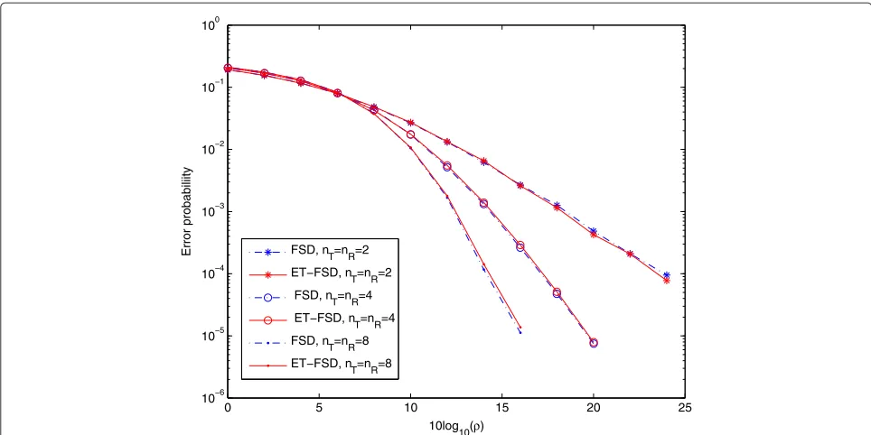
Figure 2The curves of error probability.The modulation scheme used is QPSK. The number of levels of the FE stage isp= √nT −1 for FSD,
and the initial number of levels of the FE stage isp¯= √nT −1 for ET-FSD. This figure shows the numerical result for Theorem 1.
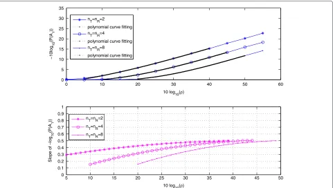
5.2 Asymptotic behavior ofP(A1)
According to Lemma 3, P(A1) tends to 0 as ρ →
+∞, which decays faster than ρ−(1−γ )(nR−nT+1). Several results of this study (including Lemma 6 and Theorems 2 and 3) are directly or indirectly affected by the asymp-totic behavior of P(A1). Hence, we pay special atten-tion to the numerical results of P(A1). In the upper subgraph of Figure 3, the curves of −10 log10(P(A1)) against 10 log10(ρ) are shown for three system deploy-ments, the slopes of which grow large and converge at some constant values as the average SNR ρ increases within the regime 0 to 60 of 10 log10(ρ). Next, we apply the Matlab tools of polynomial curve fitting to acquire the fitting curves for −10 log10(P(A1)) against 10 log10(ρ), as may be seen in the upper subgraph of Figure 3 as well. Then by computing the slopes of the fitting curves via the derivative of the functions asso-ciated with the fitting curves, the approximate slopes can be plotted as the lower subgraph of Figure 3, which approach but are not larger than (1 − γ )(nT − nR + 1) = 1/2. When−limρ→+∞loglog1010P(Aρ1) exists, the slope of the curve of −10 log10(P(A1)) against 10 log10(ρ) shall be asymptotic to −log10P(A1)
log10ρ as ρ → +∞. Since in the lower subgraph of Figure 3 the slopes are already shown to converge at a constant value 1/2, it implies that −limρ→+∞loglog1010P(ρA1) would also converge at 1/2. This is in accordance with what we can expect from Lemma 3.
5.3 Asymptotic behavior ofE(Xp(H))
As we can see in (26), E(Xp(H),j) → ζ0 asρ → +∞. Now it is verified again via Figure 4 that (26) holds true. Given this asymptotic behavior of E(Xp(H)), we would also be aware that the constraint of sum com-plexity, Cn∗, which is set as (25), converges at nζ0 + nδ at high SNR. In other words, 1nC∗n → ζ0 + δ as ρ → +∞. Thus, in this case, we can expect that the complexity constraint per user tends to ζ0 + δ as ρ increases.
5.4 Statistics ofP1nSn≥E(Xp(H),j)+δ
Based on (19) and (27), it can be found thatP(Sn∈An)≤ P1nSn≥E(Xp(H),j)+δ, where P(Sn∈An) affects the
error probability of the SCC-ET-FSD for each user as (29). Lemma 6 reveals the property ofPn1Sn≥E(Xp(H),j)+δ
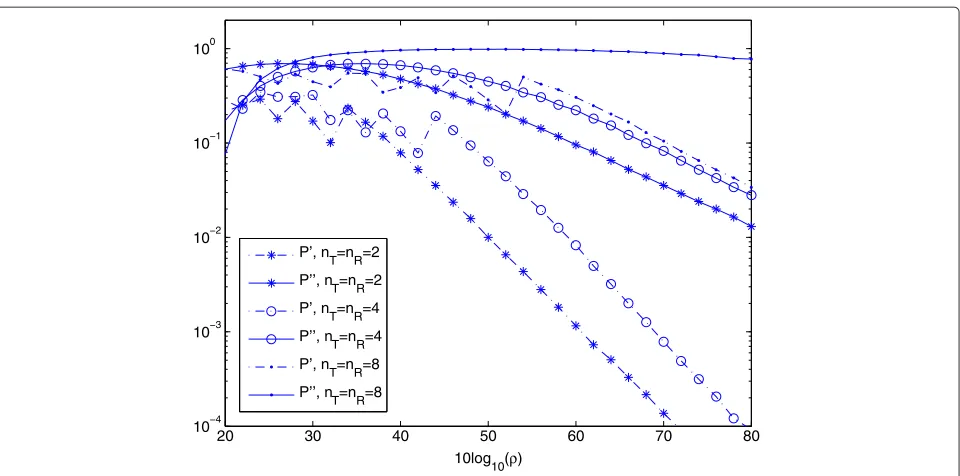
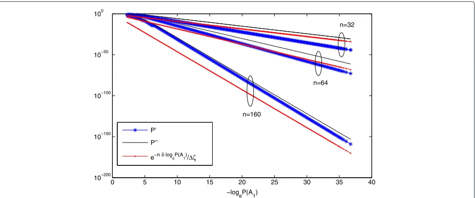
which is a key point to prove the existence of the scale effect. Therefore, we present herein the results produced by computer simulations in Figures 5 and 6, where for the purpose of notational simplification, it is defined as
PP1nSn≥E(Xp(H),j)+δ
andPe−nI(E(Xp(H),j)+δ).
In Figure 5, if 20 ≤ 10 log10(ρ) ≤ 90, the value of
0 10 20 30 40 50 60 0
5 10 15 20 25 30 35
10 log10(ρ)
−10log
10
(P(A
1
))
5 10 15 20 25 30 35 40 45 50
0 0.1 0.2 0.3 0.4 0.5 0.6 0.7 0.8 0.9 1
10 log10(ρ)
Slope of −log
10
(P(A
1
))
nT=nR=2
polynomial curve fitting nT=nR=4
polynomial curve fitting nT=nR=8
polynomial curve fitting
nT=nR=2
nT=nR=4
nT=nR=8
Figure 3The curves show the asymptotic behavior ofP(A1)with the eventA1defined as (10).The modulation scheme used is QPSK.γis set
to 1/2. The initial number of levels of the FE stage isp¯= √nT −1 for ET-FSD. This figure shows the numerical result for Lemma 3.
P = P1nSn≥E(Xp(H),j)+δ
seems to be less thanP = e−nI(E(Xp(H),j)+δ). In Figure 6, by setting n = 32, 64, or
160, the curves of P = P1nSn≥E(Xp(H),j)+δ
, P =
e−nI(E(Xp(H),j)+δ), ande−nδlogeP(A1)/ζ become closer asn increases. This is coincident with the theoretical results derived earlier.
6 Conclusion
This paper provides the insights into the scale effect of ET-FSD. Under the scale effect, the worst-case complex-ity per user of ET-FSD could decrease as the number of users increases without loss of the diversity order. Within the study, the large deviation principle is used as an
0 10 20 30 40 50 60 70 80
0 2 4 6 8 10 12 14 16
10log10(ρ)
Expectation of X
p(
H),j
ζ0
nT=nR=2
n
T=nR=4
nT=nR=8
Figure 4The expectation ofXp(H),E(Xp(H))against10 log10(ρ).The initial number of levels of the FE stage isp¯= √n
20 30 40 50 60 70 80 10−4
10−3 10−2 10−1 100
10log
10(ρ)
P’, n
T=nR=2
P’’, n
T=nR=2
P’, n
T=nR=4
P’’, n
T=nR=4
P’, n
T=nR=8
P’’, n
T=nR=8
Figure 5PPn1Sn≥E(Xp(H),j)+δ
andPe−nI(E(Xp(H),j)+δ)against10 log
10(ρ)withn=16.The initial number of levels of the FE
stage isp¯= √nT −1 for ET-FSD.
appropriate and powerful tool to prove the existence of the scale effect.
Endnotes
a Within this study, unless otherwise stated, the
complexity of MIMO detection is measured by the number of all possible candidates ofs.
b The polynomial complexity constraint stands for the
complexity constraint of MIMO detection being no more than a polynomial function in eithernTorm.
c For the multi-user scenario of MIMO system, we
assume that all users have the same number of antennas and different users operate on orthogonal resources via time division multiple access or frequency division multiple sccess technologies.
d Even if we take the length ofscandidate or the
complexity of ZF estimate into consideration, the complexity related toζ0is still polynomial.
Appendices Appendix 1 Proof of Lemma 2
Proof.It should be emphasized that, for 0 ≤j≤p−1,
A0A1· · ·Ajcan represent the event wherein Algorithm 1
encounters early termination in thejth iteration. Mean-while, the event wherein no early termination happens in Algorithm 1 can be denoted byA0A1· · ·A(p−2)A(p−1). Moreover, the events A0A1· · ·Aj with 0 ≤ j ≤ p−1
andA0A1· · ·A(p−2)A(p−1)are mutually exclusive. Then, it follows from [30] that
peSE=P(ESE,A0)+P(ESE,A0A1)+. . . +PESE,A0A1· · ·A(p−2)A(p−1)
+PESE,A0A1· · ·A(p−2)A(p−1)
,
(36)
and
peET−SE=P(EET−SE,A0)+P(EET−SE,A0A1)+. . . +PEET−SE,A0A1· · ·A(p−2)A(p−1)
+PEET−SE,A0A1· · ·A(p−2)A(p−1)
, (37)
where P(·,·) denotes the joint probability of two joint events.
Concerning the items in (36) and (37), it follows that
PEET−SE,A0A1· · ·A(p−2)A(p−1)
=P(ESE,A0A1· · ·A(p−2)A(p−1)) <peSE.
(38)
0 5 10 15 20 25 30 35 40 10−200
10−150 10−100 10−50 100
−log
eP(A1)
P’
P’’
e−n δ logeP(A1)/Δζ
n=160
n=64 n=32
Figure 6PP1nSn≥E(Xp(H),j)+δ
,Pe−nI(E(Xp(H),j)+δ)ande−nδlogeP(A1)/ζagainst−log
eP(A1).The initial number of levels of
the FE stage isp¯= √nT −1 for ET-FSD. This figure shows the numerical result for Lemma 6.
of the former is no larger than the probability of the latter, (37) leads to
peET−SE≤P
EET−SE,A0
+P(EET−SE,A1)+. . . +PEET−SE,A(p−1)
+PEET−SE,A0A1· · ·A(p−2)A(p−1)
, (39)
where because ofEET−SE=#ni=Tp+1{sai =sai},
P(EET−SE,Aj)
≤
nT
i=p+1
P(sai=sai,η(j+1)≥ρ
γ). (40)
In the above, withp+1≤i ≤nT,saiis the element of
sSE, while the correspondingsaiis the element ofsSE.
If A0A1· · ·A(j−1) happens and the ET-FSD meets η(j+1) ≥ργ, the eventAjwill occur andpwill be set toj
by Algorithm 1 before quitting the loop of preprocessing for the SE stage, i.e.,p := j. Then withp+1 ≤ i ≤ nT, letηa
idenote the post-processing SNR of the ZF estimate
for the aith transmit symbol,sai, in the SE search stage
under the conditionη(j+1) = xwithx≥ ργ. In this case, due to the definition ofη(j+1) as (5), it should be known thatη(j+1)=η(p+1) ≤ηai. Hence, there exist somex
≥x
such thatP(sai = sai|η(j+1) = x) = P(sai = sai|ηai =
x). Herein for each transmit symbol, the ZF estimate in
the SE search always utilizes the ML symbol detection. Therefore, it satisfies that
Psai=sai|η(j+1)=x
=Psai=sai|ηai=x
=NeQ ⎛ ⎝ &
xd2min
2
⎞
⎠≤Neexp
−xd2min 4
≤Neexp
−xd2min 4
,
(41)
whereNeanddminare the number of nearest neighbors and the minimum distance of separation of the underly-ing scale constellation, respectively [1,30]. To obtain the inequality of (41), the Chernoff bound has been used, i.e.,
Q(x)≤exp(−x2/2). Therefore, we can have
Psai=sai,η(j+1)≥ρ
γ
=
+∞
)
ργ
P(sai=sai|η(j+1)=x)fη(j+1)(x)dx
≤Neexp
−ργd2min 4
+∞)
ργ
fη(j+1)(x)dx
≤Neexp
−ργd2min 4
.
(42)
In view of (42), the relation of (40) may also be expressed as
P(EET−SE,Aj)≤(nT−p)Neexp
−ργd2min 4
Moreover, the combination of (43) with (38) and (39) leads to
peET−SE≤p(nT−p)Neexp
−ργdmin2 4
+P(EET−SE,A0A1· · ·A(p−2)A(p−1))
≤p(nT−p)Neexp
−ργd2min 4
+peSE.
(44)
By combining (9) and (44), we can conclude that set-ting the judging criterion for early termination as (8) is reasonable sinceργ with 0 < γ < 1 can make the rela-tions in (9) and (44) able to simultaneously establish tight upper bounds (which decay rapidly asρincreases) for the associated probabilities,P(η(j+1)< ργ)andpeET−SE.
Therefore, Lemma 2 is verified.
Appendix 2
Background knowledge of diversity order
Definition 3.Suppose there is a function f(ρ). The symbol =. is always employed to simplify the expres-sions of exponential equality as f(ρ) =. ρ−d ⇔ limρ→+∞loglogf(ρ)ρ = −d. If f(ρ)is the error probability of
some MIMO detector andρdenotes average received SNR, d will be the diversity order [27].
Meanwhile, the notation ˙≤and<˙ follow after replacing =with≤and<in above the definition, respectively.
Lemma 8.With the functions f1(ρ)=. ρ−d1and f2(ρ)=. ρ−d2, for f(ρ)=f
1(ρ)+f2(ρ), it is established that
f(ρ)=. ρ−min(d1,d2), (45)
wheremin(·,·)returns the minimum of two inputs.
Proof.Without loss of generality, we assume d1 ≥ d2. Thus,
lim ρ→+∞
logf(ρ)
logρ =ρ→+∞lim
log(f1(ρ)+f2(ρ)) logρ
= lim ρ→+∞
logf2(ρ) logρ
+ lim ρ→+∞
log(1+f1(ρ)/f2(ρ)) logρ = −d2= −min(d1,d2).
Lemma 9.Having f1(ρ) =. ρ−d1 and f2(ρ) =. ρ−d2, if f1(ρ)≤f2(ρ)for0< ρ <+∞, it will hold true that
d1≥d2. (46)
Proof.We can prove (46) byd1= −limρ→+∞ loglogf1(ρ)ρ ≥ −limρ→+∞loglogf2(ρ)ρ =d2.
Appendix 3 Proof of Theorem 1
Proof.Recalling from (4), keeping (13) in mind and utilizing (45) and (46), we get
min(dML,dET−SE)≤dET−FSD≤dML=nR, (47)
wheredET−FSD ≤ dMLis true because the ML detector has the optimal performance. Thus, the diversity order of the ET-FSD will not go beyond that of the ML detector.
Once more applying (45) and (46) to (44), the following can be obtained:
dET−SE≥min(+∞,− lim ρ→+∞
logpeSE
logρ ). (48)
SincepeSE corresponds to the probability of the error eventsSE = sSE in the FSD (or equivalently, the ET-FSD without early termination), by referring to [9], we get −limρ→+∞loglogpeρSE = (nR−nT)(p+1)+(p+1)2. With the special setting ofpas (3), it is true that(nR−nT)(p+ 1)+(p+1)2≥nR.
Therefore, (48) yields dET−SE ≥ nR, and (47) finally reduces to
dET−FSD=nR. (49)
We can conclude that the ET-FSD is able to achieve full diversity.
Appendix 4 Proof of Lemma 3
Proof.For (14), as the event ζp(H) = ζ0 is identical to another event η1 ≥ ργ according to (10), we can get
P(ζp(H) = ζ0) = P(A1) = 1−P(A1). Due to Lemma 1, P(A1)→0 orP(A1)→1 asρ→ +∞.
Then taking the logarithm of (9) and then dividing by logρ, we could derive (15).
For (16), the expectation ofζp(H)can be given by
Eζp(H)
=PA0
ζ0+PA0A1
ζ1+. . . +PA0A1· · ·A(p−2)A(p−1)
ζ(p−1) +PA0A1· · ·A(p−2)A(p−1)
ζp ≤PA0ζ0+P(A0)ζ1+. . .
+P(A(p−2))ζ(p−1)+P(A(p−1))ζp.
Appendix 5 Proof of Lemma 5
Proof. Given the definition of (18) and (20), we get
ϕ(t)=P(Xp(H),j=ζ0)etζ0+P(Xp(H),j=ζp)etζp. (50)
Incorporating ϕ(t) of (51) into (53) and organizing the items, we have δ[1 − P(A1)]+δP(A1)et(ζp−ζ0) =
Investigating the second derivative of f(t), it can be obtained that
Hence, it is apparent that the critical point obtained by (54) yields the maximum value off(t), which can be
It should be clear from a look at the items on the right-hand side of the second equality in (55) that [1−
P(A1)]ζ0t+P(A1)ζpt+δt= P(A1)(ζp−ζ0)t+ζ0t+δt. It can also be observed that log([1−P(A1)]+P(A1) etζ=log1+P(A
1)(etζ −1).
By replacing t with the critical point of (54), we get log([1−P(A1)]+P(A1)etcpζ)=log(ζ[1ζ[1−−P(PA(A1)1])−]δ).
Therefore, the exact expression of the maximum value off(t), i.e.,fmax, is eventually obtained by (55). By recalling (22), (52), and (55), we obtainIEXp(H),j
+δ=fmax. Thus, the validation of Lemma 5 is established.
Appendix 6 Proof of Lemma 7
Proof. Based on the conclusion of (49), it follows that
P(EET−FSD,k)=. ρ−nR.
Then in view of (28), (45), and (46), it suffices to show thatPEET−FSD,k|Sn∈An
PSn∈An
˙≤ρ−nR.
Provided that, when Sn ∈ An, no detection
out-age occurs, which means that the sum complex-ity constraint has no effect on the detected result, it is true that PEET−FSD,k|Sn∈An
≤1, together with (23) and (57), it is established that
PESCC∗ −ET−FSD,k|Sn∈An
Competing interests
The authors declare that they have no competing interests.
Acknowledgements
The authors wish to thank the anonymous reviewers for their helpful comments and their thoughtful reviews. They greatly improved the quality of the paper. A short version of this paper was presented at the IEEE PIMRC 2012. This work is sponsored by the BUPT Innovative Funds for Young Scholars (2012RC0507 and 2013RC0210), National Science and Technology Major Projects under grants 2012ZX03003011, 2012ZX03003007 and
2013ZX03003012, National Natural Science Foundation of China under grant nos. 60572120, 61001117, and 60602058, the National Key Basic Research Program of China (973 Program) under grant no. 2009CB320400, and the Joint Funds of NSFC-Guangdong under grant U1035001.
Author details
1Automation School, Beijing University of Posts and Telecommunications
(BUPT), Beijing 100876, China.2Electronic School, Beijing University of Posts and Telecommunications (BUPT), Beijing 100876, China.3Wireless Signal Processing and Network Lab (Key Lab. of Universal Wireless Communication, Ministry of Education), Beijing University of Posts and Telecommunications (BUPT), Beijing 100876, China.
Received: 8 January 2013 Accepted: 12 June 2013 Published: 3 July 2013
References
1. A Paulraj, R Nabar, D Gore,Introduction to Space-Time Wireless
Communications, 1st edn. (Cambridge University Press, Cambridge, 2003) 2. U Fincke, M Pohst, Improved methods for calculating vectors of short
length in a lattice, including a complexity analysis. Math. Comp. 44, 463–471 (1985)
3. E Viterbo, J Boutros, A universal lattice code decoder for fading channels. IEEE Trans. Inform. Theory.45(5), 1639–1642 (1999)
4. E Agrell, T Eriksson, A Vardy, K Zeger, Closest point search in lattice. IEEE Trans. Inform. Theory.48(8), 2201–2214 (2002)
5. B Hassibi, H Vikalo, On the sphere-decoding algorithm I. Expected complexity. IEEE Trans. Signal Process.53, 2806–2818 (2005) 6. A Wiesel, YC Eldar, S Shamai, Semidefinite relaxation for detection of
16-QAM signaling in MIMO channels. IEEE Signal Process. Lett.12(9), 653–656 (2005)
7. K Lee, J Chun, ML symbol detection based on the shortest path algorithm for MIMO systems. IEEE Trans. Signal Process.55(11), 5477–5484 (2007) 8. Z Guo, P Nilsson, Algorithm and implementation of the K-best sphere
decoding for MIMO detection. IEEE J. Select. Areas Commun.24(3), 491–503 (2006)
9. LG Barbero, JS Thompson, inProceedings of IEEE International Conference on Acoustics, Speech and Signal Processing 2006. Performance analysis of a fixed-complexity sphere decoder in high-dimensional MIMO systems (IEEE New York, 2006), pp. 14–19
10. B Gestner, X Ma, DV Anderson, Incremental lattice reduction: motivation, theory, and practical implementation. IEEE Trans. Wireless. Communi. 11(1), 188–198 (2012)
11. D Wubben, D Seethaler, J Jalden, G Matz, Lattice reduction. IEEE Trans. Wireless. Communi.28(3), 70–91 (2011)
12. JW Choi, B Shim, AC Singer, NI Cho, Low-complexity decoding via reduced dimension maximum-likelihood search. IEEE Trans. Signal Process.58(3), 1780–1793 (2010)
13. J Jalden, P Elia, Sphere decoding complexity exponent for decoding full rate codes over the quasi-static MIMO channel. IEEE Trans. Inform. Theory. 58, 5785–5803 (2012)
14. W Abediseid, M Damen, Lattice sequential decoder for coded MIMO channel: performance and complexity analysis. IEEE Trans. Inform. Theory (2010). doi:10.1109/ISIT.2010.5513497
15. J Goldberger, A Leshem, MIMO detection for high-order QAM based on a Gaussian tree approximation. IEEE Trans. Inform. Theory.57(8), 4973–4982 (2011)
16. J Jalden, B Ottersten, On the complexity of sphere decoding in digital communications. IEEE Trans. Signal Process.53(4), 1474–1484 (2005)
17. J Jalden, LG Barbero, B Ottersten, JS Thompson, The error probability of the fixed-complexity sphere decoder. IEEE Trans. Signal Process.57(7), 2711–2720 (2009)
18. J Jalden, B Ottersten, inProceedings of International Symposium on Information Theory 2005. On the limits of sphere decoding (IEEE New York, 2005), pp. 1691–1695
19. M Taherzadeh, AK Khandani, On the limitations of the naive lattice decoding. IEEE Trans. Inform. Theory.56(10), 4820–4826 (2010) 20. R Qian, Y Qi, T Peng, W Wang, J Yang, On the scale effects oriented MIMO
detector: diversity order, worst-case unit complexity and scale effects. Elsevier Signal Process.93(1), 277–287 (2013)
21. R Qian, Y Qi, T Peng, W Wang, inProceedings of the IEEE Globecom 2012 Workshop on Cloud Base-Station and Large-Scale Cooperative Communications. Exploiting scalar effects of MIMO detection in cloud base-station: feasible scheme and universal significance (IEEE New York, 2012), pp. 216–221
22. J Jalden, L Barbero G, B Ottersten, JS Thompson, inProceedings of IEEE International Conference on Acoustics, Speech and Signal Processin 2007. Full diversity detection in MIMO systems with a fixed-complexity sphere decoder (IEEE New York, 2007), pp. III-49
23. D Gore, RW Heath Jr., A Paulraj, inProceedings of the IEEE International Symposium on Information Theory 2002. On performance of the zero forcing receiver in presence of transmit correlation (IEEE New York, 2002), p. 159
24. R Narasimhan, Spatial multiplexing with transmit antenna and constellation selection for correlated MIMO fading channels. IEEE Trans. Signal Process.51(11), 2829–2838 (2003)
25. H Lutkepohl,Handbook of Matrices. (Wiley, Chichester, 1996) 26. A Khoshnevis, A Sabharwal, inProceedings of the Allerton Conference on
Communication, Control and Computing. On diversity and multiplexing gain of multiple antenna systems with transmitter channel information (University of Illinois Monticello, 2004)
27. L Zheng, D Tse, Diversity and multiplexing: a fundamental tradeoff in multiple-antenna channels. IEEE Trans. Inform. Theory.49(5), 1073–1096 (2003)
28. Economies of scale. (Wikipedia, 2013). http://en.wikipedia.org/wiki/ Economies_of_scale. Accessed 1 Feb 2013
29. F Hollander,Large Deviations. (American Mathematical Society, Providence, 2008)
30. J Proakis G,Digital Communications, 4th edn. (McGraw-Hill, New York, 1995)
31. SM Ross,A First Course in Probability, 8th edn. (Pearson Education, Upper Saddle River, 2009)
doi:10.1186/1687-6180-2013-125
Cite this article as:Qianet al.:Scale effect analysis of early-termination fixed-complexity sphere detector.EURASIP Journal on Advances in Signal Processing20132013:125.
Submit your manuscript to a
journal and benefi t from:
7Convenient online submission
7Rigorous peer review
7Immediate publication on acceptance
7Open access: articles freely available online
7High visibility within the fi eld
7Retaining the copyright to your article