The Cramer-Rao Bound and DMT Signal Optimisation
for the Identification of a Wiener-Type Model
H. Koeppl
Christian Doppler Laboratory for Nonlinear Signal Processing, Graz University of Technology, 8010 Graz, Austria Email:[email protected]
A. S. Josan
Department of Electronics and Communication Engineering, Indian Institute of Technology Guwahati, Guwahati 781039, Assam, India
Email:[email protected]
G. Paoli
System Engineering Group, Infineon Technologies, 9500 Villach, Austria Email:[email protected]
G. Kubin
Christian Doppler Laboratory for Nonlinear Signal Processing, Graz University of Technology, 8010 Graz, Austria Email:[email protected]
Received 2 September 2003; Revised 8 January 2004
In linear system identification, optimal excitation signals can be determined using the Cramer-Rao bound. This problem has not been thoroughly studied for the nonlinear case. In this work, the Cramer-Rao bound for a factorisable Volterra model is derived. The analytical result is supported with simulation examples. The bound is then used to find the optimal excitation signal out of the class of discrete multitone signals. As the model is nonlinear in the parameters, the bound depends on the model parameters themselves. On this basis, a three-step identification procedure is proposed. To illustrate the procedure, signal optimisation is explicitly performed for a third-order nonlinear model. Methods of nonlinear optimisation are applied for the parameter estimation of the model. As a baseline, the problem of optimal discrete multitone signals for linear FIR filter estimation is reviewed.
Keywords and phrases:Wiener model, Cramer-Rao bound, signal design, nonlinear system identification.
1. INTRODUCTION
In the design of optimal excitation signals for system iden-tification, the Cramer-Rao bound plays a central role. For a given model structure, it gives a lower bound on the vari-ance of the unbiased model parameter estimates for a given perturbation scenario [1]. The problem of signal optimisa-tion for the identificaoptimisa-tion of linear models is considered in [2]. We focus on a nonlinear model structure proposed in [3], which is nonlinear in the parameters and can be consid-ered a generalisation of the classical Wiener model [4, page 143]. For the classical Wiener model, the Cramer-Rao bound was derived in [5]. The goal of this work is to gain further insight into the design of optimal excitation signals for the identification of nonlinear cascade systems. The application that drove our investigations is adaptive nonlinear filtering
for ADSL data transmission systems. The block diagram in
Twisted wire
pair Hybrid
Receive path
−
Nonlinear
echo canceler ADSL digitaltransceiver
Transmit path Nonlinear
line driver
Figure1: Block diagram of the application of a nonlinear canceler of the hybrid echo for an ADSL transceiver system.
tones in the input signal and of a finite number of samples for the estimation of the model parameters.
The work is organised as follows. InSection 2, the con-sidered Wiener-type model is derived from the general Volterra model. The Cramer-Rao bound for this model is computed in Section 3 while Section 4 deals with the pa-rameter estimation algorithm. Verification of the derived Cramer-Rao bound via numerical simulations is performed in Section 5. A discussion, new algorithms, and simulation results concerning the design of optimal excitation signals for the considered model are given inSection 6.
2. VOLTERRA MODEL AND THE WIENER-TYPE MODEL
The multivariate kernelvp[k1,. . .,kp] of the homogeneous
Volterra system ofFigure 2with
y[n]= Mp−1
k1=0 · · ·
Mp−1
kp=0
vpk1,. . .,kpun−k1
· · ·un−kp
(1) is factorisable if it can be written as a product of lower-dimensional terms
vpk1,. . .,kp
=rpk1,. . .,kr
wpkr+1,. . .,kp
(2)
shown inFigure 3. The kernel function is fully factorisable if its kernelvp[k1,. . .,kp] can be written as
vpk1,. . .,kp
=
p
i=1
hpiki. (3)
The corresponding block diagram is depicted in Figure 4. If all one-dimensional kernels hpi[ki] are identical, that is, hp[ki]=hpi[ki] fori=1,. . .,pwith
vpk1,. . .,kp= p
i=1
hpki, (4)
one arrives at the cascade structure of Figure 5, which is recognised as a homogeneous Wiener system. In the case of a general Volterra system of order N for which condi-tion (4) holds for all orders p with p = 1,. . .,N, we ob-tain the considered simplified factorisable Volterra system.
u[n]
vp[k1,. . .,kp] y[n]
Figure2: Homogeneous Volterra system of orderp.
u[n]
rp[k1,. . .,kr]
wp[kr+1,. . .,kp]
y[n]
Figure3: Partially factorisable homogeneous Volterra system of or-derp.
u[n]
hp1[k1]
hp2[k2] . . .
hp(p−1)[kp−1]
hpp[kp]
y[n]
Figure4: Fully factorisable homogeneous Volterra system of order
p.
This Wiener-type model and the related measurement sce-nario are depicted inFigure 6. If theNdifferent linear kernels hp[k] inFigure 6differ only by a scaling factor, the classical Wiener model is obtained. The measured outputz[n] of the considered model can be written asz[n]=y[n] +[n] with
y[n]=N p=1
Mp−
1
k=0
hp[k]u[n−k] p
, (5)
u[n]
hp[k] (·)p y[n]
Figure5: Homogeneous Wiener system of orderp.
u[n]
Figure6: The considered nonlinear Wiener-type model.
loss of generality, Mp = M for p = 1,. . .,N is assumed. For convenience, the following objects are defined. The linear kernel matrixH∈RM×Nis defined as considered observation sample length or estimation horizon. To be precise, to build up anNs×Mdata matrixU, one re-quires the knowledge ofNs+M−1 samples of the input signal u[n], which would actually be the estimation horizon. Nev-ertheless, in the following, we stick to the convention that the estimation horizon is the number of rows of the data matrix U, that is,Ns. In addition, the power operator P :Rn×m→Rn
is defined, where the notation (·)I, denoting one element of a nonscalar object withI possibly a multi-index, was used. Making use of the above definitions, the output of the non-linear model ofFigure 6reads
z=PX+, X=UH, (9)
where the elements of this objects correspond tozn ≡z[n], n ≡ [n], and Xnp ≡ xp[n]. The parameter vectorθ ≡
vec(H) will be needed in the following, where the linear index
jofθj corresponds to the matrix indices [k,p] ofHkp with j =(p−1)M+kandk= jmodM,p= j/M, where· denotes the ceiling function.
3. THE CRAMER-RAO BOUND FOR
THE WIENER-TYPE MODEL
The Cramer-Rao bound is the theoretical lower bound for the variance of all unbiased estimators ˆθfor the model pa-rametersθand is determined by the diagonal elements of the inverse of the Fisher information matrixF:
Fij≡E
Here E(·) denotes the expectation operator with respect to the random vector z= PX+andl(θ|z) is the likelihood function for the parameter vectorθgiven the noisy observa-tion vectorz[1]. Thus,
covθθTij≡Eθi−Eθiθj−Eθj≥F−1
ij.
(11)
Under the regularity condition [6, page 26]
E
the Hessian matrix of the objective function−lnl(θ|z) for the maximum likelihood estimation. For the additive Gaus-sian noise model of, the likelihood functionl(H|z) for the parameter matrixHgiven the observation vectorzreads as follows:
The entries of the Fisher information matrix (10) for the con-sidered Wiener-type model (5) are calculated as follows. The log-likelihood function reads as follows:
lnlH|z= −1
∂lnlH|z
been introduced. The first two terms of the product give
∂lnlH|z
where (·)[p] means elementwise operation. The last term
yields
Applying the expectation operator to the above expression gives the desired result for the Fisher information matrix, which reads For the special case of a linear FIR filter, that is,N =1, the Fisher information matrix reads, using (19),
F=F˜11=UTΣ−1U, (25)
which, forΣ=σ2I, gives the familiar result [1, page 86]
F−1=σ2UTU−1 (26)
for the Cramer-Rao bound for linear FIR filters.
4. PARAMETER ESTIMATION
For parameter estimation, the likelihood functionl(θ|z) is maximised with respect to θ using methods of nonlinear optimisation. The optimisation problem is given as
ˆ (14) can be computed explicitly. Following the matrix nota-tion for the model parameters, the gradient can be written in matrix form. Define the gradient matrix∂Has composed of the gradient vectors for each order of nonlinearity
∂H≡ objective functionJ(θ), the elements are found to be
∂hsJ(H)= −UTX˜sΣ−1. (29)
In correspondence to the matrix structure of the Fisher in-formation matrix in (24), the “off-diagonal” submatrices of the Hessian matrix are
Gsp≡∂hshTpJ(H)=UTX˜sΣ
−1X˜
pU fors=p. (30)
The diagonal submatrices given in component notation read
G[rs][qs]≡∂HrsHqsJ(H) that is a zero-mean process, the Fisher information ma-trix (24) is retained. As with (29), (30), and (31), first- and second-order derivatives are available, and it is possible to apply a Newton-like optimisation algorithm [7] for the min-imization of (27). This algorithm uses the quadratic approx-imation ofJ(θ) around some estimateθ(k)obtained afterk
proximation is minimised with respect toδ, whereg(k)and
G(k) denote the gradient and Hessian evaluated atθ(k)
, re-spectively. For this task, the Matlab routine fminunc.m [8] is applied. This procedure requires good initialisation to con-verge to the global minimum of the objective functionJ(θ) which is in general multimodal. In this case, the maximum likelihood estimator (27) yields an unbiased estimate. Fur-thermore, the maximum likelihood estimator is a minimum variance estimator [1], thus the variance of this estimator co-incides with the Cramer-Rao bound.
5. VERIFICATION OF THE THEORETICAL RESULT
Table1: Model coefficients of the third-order Wiener-type reference model of the line-driver circuit.
Tap k=0 k=1 k=2 k=3 k=4 k=5
h1[k] 4.2299 1.3909 −1.0805 0.7283 −0.3481 0.0931
h3[k] 0.0511 0.1537 −0.2463 0.1418 −0.0314 0.0009
0 0.2 0.4 0.6 0.8 1
Normalised frequency (xπ)
−5
Figure7: Absolute value of the linear transfer functionH1(ejω) of the Wiener-type reference model ofTable 1.
variance obtained from the Fisher information matrix (24) with the parameter variance obtained by repeated estima-tion of the model parameters with the algorithm described inSection 4. As this estimator is a minimum variance esti-mator, the two variances are expected to match. This coinci-dence is checked for DMT input signals as well as for white Gaussian noise (WGN) input signals over different signal-to-noise (SNR) levels.
5.1. The reference model
For the simulation, a specific reference configuration of the Wiener-type model is chosen. This reference configuration is a simple discrete-time model of an ADSL, G.Lite line-driver circuit [9]. To present reproducible results, the sim-plest model of the circuit was chosen as the reference model and explicit values of the model coefficients are given. It is a third-order model encompassing 12 coefficientsθj. Through the differential design of the circuit, the effects of nonlineari-ties of even orders are negligible compared to the effects of the nonlinearities of odd orders. Thus, the model consists only of a dominating linear part withM1=6 and of a small
part of third order withM3 = 6. The explicit values of the
model coefficients are given inTable 1. They were found orig-inally by identifying the line-driver circuit using a broadband DMT input signal and the estimation algorithm ofSection 4.
The model equation for this case reads
z[n]=
Normalised frequency (xπ)
−25
Figure8: Absolute value of the cubic transfer functionH3(ejω) of the Wiener-type reference model ofTable 1.
Written in the compact notation ofSection 3, this gives
z=PUHr+, (34)
with the reference coefficient matrixHr ∈R6×2. Frequency
responses for the linear partH1(ejω)=F(h1[k]) and for the
cubic partH3(ejω) = F(h3[k]) of the reference model are
depicted in Figures7and8, respectively. The linear response shows the typical lowpass characteristic of a power amplifier, while the third-order response reflects the common observa-tion that the nonlinear distorobserva-tion gets higher for higher fre-quencies. InFigure 9, the power spectrum of the output sig-nal of the Wiener-type reference model ofTable 1is shown, for a typical downstream ADSL DMT signal as input. The magnitude of the intermodulation products indicates that the nonlinear distortion introduced by the third-order term is 60 dB below the carrier signal. Thus, we are dealing with an extremely weak nonlinear system. Subsequently, the Fisher information matrix of (24) and its inverse are computed for this reference model. In correspondence to the partitioning (24) of the Fisher information matrix
F=σ2
0 0.2 0.4 0.6 0.8 1
Figure9: Power spectrum of the output of the Wiener-type refer-ence model of Table 1for the line-driver circuit: DMT input sig-nal withNc =95 carriers; the perturbation is additive WGN with
σ2=1×10⁻⁵.
Figure10: Cramer-Rao lower bound on the parameter covariance matrix cov(θθT)ijwithM=6, first- and third-order nonlinearity, andNs =1000; the pertubation is WGN withσ2 =1×10⁻⁵and
u[n] is a WGN input signal with powerσ2 u=0.64.
In Figure 10, the parameter covariance matrix cov(θθT)ij for the Wiener-type reference model is shown for the case Ns=1000 andσ2 =1×10⁻⁵for a WGN input signal with
varianceσ2
u=0.64. The figure reveals that there is a high
co-variance between the linear parameters and the third-order parameters. That corresponds to the known fact that even in the case of a white input signal, the homogeneous first-and third-order responses of a multilinear operator, such as a Volterra model, are correlated [10].
5.2. Parameter estimation and variance comparison In the following, the derivation of Section 3is verified us-ing different excitation signals and different perturbation scenarios. These investigations of the Wiener-type reference model of Table 1 are done with an estimation horizon of Ns = 50. The variance estimates of the estimators are
ob-tained by repeating the identification procedure ofSection 4
30 40 50 60 70 80 90
Figure11: Linear dependence of Cramer-Rao bound (dashed) on the SNR and variance of the estimators (solid) over different SNR with 95% confidence intervals shown as vertical bars, plotted for one kernel value for each orderp; the two upper curves correspond to parameterH12=h3[0]; the two lower curves correspond to pa-rameterH11=h1[0]; the input signal is WGN.
forNr = 100 i.i.d. realisations of the perturbation process [n]. Following the asymptotic results of the normality of the maximum likelihood estimator [11, page 52], the parameter estimates pass the Lilliefors test for normality [12]. Thus, the 95% confidence intervals of a normal distribution are indi-cated in the following figures. To keep these figures simple, the Cramer-Rao bound diag(F−1) and the variance estimates
var(θ) of only one model parameter per order of nonlinearity pare shown versus different SNR.
5.2.1. WGN input signal
The input signalu[n] to the reference model is taken to be WGN, u[n] ∼ N(0,σ2
u) withσu2 =0.64, while the additive
perturbation of the output y[n] is[n] ∼ N(0,σ2). The
Cramer-Rao bound, the variance estimates of the estimators, and their corresponding confidence regions versus different SNR levels are given inFigure 11. Good agreement between simulation and theory can be observed.
5.2.2. DMT input signal
As a second scenario, the input signalu[n] is taken to be a DMT signal:
whereω0 is the normalised grid frequency of the DMT
sig-nal. For further use, we define the vector of amplitudes a ≡ [a0,. . .,aNc−1]T, the corresponding vector of powers
of the individual tones p, and the vector of normalised fre-quenciesω ≡ ω0·[ks,ks+ 1,. . .,ks+Nc−1]T. The phase
set ϕ ≡ [ϕ0,. . .,ϕNc−1]T for this simulation is initialised
30 40 50 60 70 80 90
Figure12: Linear dependence of Cramer-Rao bound (dashed) on the SNR and variance of the estimators (solid) over different SNR with 95% confidence intervals shown as vertical bars, plotted for one kernel value for each orderp; the two upper curves correspond to parameterH12=h3[0]; the two lower curves correspond to pa-rameterH11=h1[0]; the input signal is a DMT signal withNc=12.
performed usingNc=12 tones and is done for different SNR levels. The Cramer-Rao bound, the variance estimates of the estimators, and their corresponding confidence regions ver-sus different SNR levels are given inFigure 12. Once again, good agreement between simulation and theory can be ob-served.
6. DESIGN OF OPTIMAL EXCITATION SIGNALS
Given a model structure with unknown parameters, the ac-curacy of the parameter estimates of the model depends on the used identification procedure and on the used excita-tion signal. If the estimator is a minimum variance estimator, then its parameter variance achieves the lower bound, that is, the Cramer-Rao bound. Thus, to even further decrease the variance of the minimum variance estimator of Section 4, one can only optimise the excitation signal in such a way that the corresponding Cramer-Rao bound is decreased. To have an optimality measure, a scalar objective functionΨ :
RMN×MN →RofF−1has to be found. In the theory of
exper-iment design [13], different types of this objective function
Ψ(·) are considered. The most popular criterion of optimal-ity isΨ(F−1)= |F−1| = |F|−1, where| · |denotes the
deter-minant of a matrix.
6.1. Signal design for linear FIR filters
In this section, the well-known problem of optimising the amplitude distribution of a DMT signal subject to a total power constraint so as to achieve minimal variance estimates of the parameters of a linear FIR filter is reviewed. For a WGN perturbation, the Fisher information matrix for the linear FIR filter case is given by (26). As mentioned earlier, one way to minimize the Cramer-Rao bound is to maximize the de-terminant ofF. We apply the inequality logx≤αx−1−logα for every α > 0 to the M eigenvalues λk of the
positive-semidefinite matrixF:
Inequality (38) is equivalent to
log|F| ≤αTr(F)−M(1 + logα), (39)
with Tr(·) denoting the trace of a matrix. The quantity log|F|
reaches its upper bound atλk =λ =1/αfork =1,. . .,M. The consequences of this relation for signal optimisation are outlined in the following example. Consider the caseNsis the period of the DMT signal (37). The diagonal elements of Fare all equal and correspond to the constrained total power of the DMT signal, that is, Tr(F)=σ−2MN
spk. Thus, for
a given power of the DMT signal, the right-hand side of (39) is fixed and gives the upper bound for log|F|. It reaches its upper bound if the eigenvalues are all equal toλ=1/αwith α=σ2/(N
spk).
Furthermore, if we assume thatMis even andM =Ns,
with (7) and (26), the matrixFturns out to be a circulant. Thus, the similarity transformation which diagonalises Fis the discrete Fourier transform (DFT) T ∈ CM×M and the
eigenvalues ofFare the diagonal elements ofS=TFT−1[14,
page 379]. If the frequency spacing of the DMT signal (37) is chosen to beω0 =2π/Mandks=0, the eigenvalues ofF
correspond to the discrete power spectrum of the DMT sig-nal. The matrixFis nonsingular fork = 0,. . .,M/2, which corresponds toNc=M/2 + 1 tones of the DMT signal. The tones atk =0 andk = M/2 contribute one spectral com-ponent to the discrete power spectrum each, while all other tones contribute two spectral components each. Thus, the eigenvalues of Fare all equal and log|F| reaches its upper bound if theM/2 + 1 element amplitude vector of the DMT signal has the forma=[a/2,a,. . .,a,a/2]T. This is in accor-dance with the engineering intuition that for a finite number of tones and a predetermined power of the DMT signal, the most accurate parameter estimation is possible if the power is equally distributed over all spectral components. Note that the above example is constructed in such a way that the fre-quency grid of the DMT signal spans the full bandwidth, that is,ω=2π/M·[0, 1,. . .,M/2]T. In general, the circularity ofF is preserved ifNs=mNpandM=Np, whereNpis the period of the DMT signal andm∈N. In such situations, everymth spectral component of the DMT signal (37) withω0=2π/M
andNc =M/2 + 1 is nonzero and corresponds to an eigen-value of the matrixF. From above considerations, it is clear that for a frequency spacingω0 =2π/MandNc < M/2 + 1,
at least one eigenvalue ofFis exactly zero. Thus, the corre-sponding estimation problem is an ill-posed one. As soon as the constraintsNs/M∈Nandω0 =2π/Mdo not hold, the
0 0.2 0.4 0.6 0.8 1 Normalised frequency (xπ)
0 0.1 0.2 0.3 0.4 0.5 0.6 0.7 0.8
A
m
plitude
Figure13: Optimal amplitude distribution of a DMT signal over the full bandwidth [0,π] encompassingNc =4 tones for the esti-mation of anM=6 FIR filter.
In [15], it is shown that, for linear FIR filters, the max-imization of log|F| subject to the signal power constraint
pk ≤ 1 leads to a semidefinite programming problem
which can be solved efficiently [16]. More explicitly, the semidefinite program takes the form
max
p logF(p), subject toF(p)≥0, ˜p≥0, (40)
with ˜p ≡ [1−pk,p0,. . .,pNc−1]T. The key observation
that allows this elegant formulation is that the Fisher infor-mation matrix for a period of a DMT signal is the weighted sum of partial Fisher information matrices corresponding to each tone of the DMT signal. The weights turn out to be the powers pkof the individual tones. Following this approach, the optimal excitation signals for a linear FIR filter are found subsequently. From (25), it is clear that the amplitude distri-bution of the optimal DMT signal does not depend on the model parameters. In correspondence to the linear part of the reference model ofTable 1, the optimal amplitude distri-bution for anM=6 linear FIR filter is computed.
6.1.1. DMT signal with bandwidth[0,π]
To guarantee that the matrixFis nonsingular, above consid-erations suggest that at least Nc = M/2 + 1 = 4 tones are required if tones at ω = 0 and ω = π are included. The optimised amplitude distribution found by semidefinite pro-gramming is given inFigure 13. This amplitude distribution corresponds to a flat signal spectrum because the spectral components for ωk = 0 and ωk = π scale differently (by a factor of 2) than the other components. Thus for a finite number of tones and finite sample lengthNsequal to the pe-riod of the signal and for full bandwidth, the spectrum of the optimal DMT signal turns out to be flat. For many ap-plications, the number of tones of the excitation signal is not exactlyNc =M/2 + 1, but higher. Also for such a case with Nc> M/2+1, the optimal amplitude distribution over the full
bandwidth [0,π] is found to be spectrally flat. More interest-ing observations can be made for a bandpass DMT signal in the next section.
0 0.2 0.4 0.6 0.8 1
Normalised frequency (xπ) 0
0.1 0.2 0.3 0.4 0.5 0.6 0.7 0.8
A
m
plitude
Figure 14: Optimal amplitude distribution for a bandpass DMT signal encompassingNc =3 tones for the estimation of anM=6 FIR filter.
0 0.2 0.4 0.6 0.8 1
Normalised frequency (xπ) 0
0.1 0.2 0.3 0.4 0.5 0.6 0.7 0.8
A
m
plitude
Figure15: Amplitude distribution of a bandpass DMT signal en-compassingNc=12 tones for the estimation of anM=6 FIR filter: optimised signal (circles) and, for reference, the spectrally flat signal (crosses).
6.1.2. DMT signal with bandwidth(0,π/2)
0 1 2 3 4 5 6 7
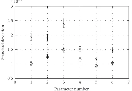
Figure16: Mean and 95% confidence region of the estimated stan-dard deviation of the linear FIR filter parameter estimates for a bandpass input signal withNc=12 tones: spectrally flat amplitude distribution (crosses), optimised amplitude distribution (circles); the perturbation is WGN withσ2 = 1×10⁻⁵and the estimation horizon isNs=56.
optimalNc =12 DMT signal and the spectrally flatNc=12 DMT signal.
6.1.3. Comparison of the estimation performance of bandpass DMT signals
Now that the optimal bandpass input signal for a linear FIR filter is found, the signal can be applied to the identification of a given linear FIR filter. The result is then compared with the identification result obtained by applying the bandpass signal with a flat spectral distribution for the given band-width (0,π/2). For this, the linear part of the Wiener-type model of Table 1 is used as the reference linear FIR filter and input-output data, that is,{u[n],z[n]}, are measured. For identification the unbiased minimum variance estimator (UMVE) [1, page 87] for the linear FIR filter case,
ˆ
θ=UTU−1UTz (41) is applied both for the optimal bandpass sequence and for the spectrally flat bandpass sequence. The variance of the es-timate ˆθis computed by performing the estimation (41) over Nr = 1000 i.i.d. noise realisations of the perturbation
pro-cess [n] ∼ N(0,σ2) with σ2 = 1×10⁻⁵ andN
s = 56.
The estimated standard deviations of each FIR filter param-eter are shown for these signals in Figure 16. In addition, the Cramer-Rao bounds for both signals and each parame-ter are computed. All bounds lie in the indicated 95% con-fidence region. To keep the figure simple, the bounds are not shown in Figure 16. The result shows clearly that the optimised DMT signal which is not spectrally flat outper-forms the spectrally flat reference DMT signal. The relative reduction of the parameter variance averaged over all FIR fil-ter paramefil-ters comes out to be 26.01% or 1.45 dB. The fol-lowing remarks can be made.
(1) To be able to apply semidefinite programming, the estimation horizonNshas to match multiples of the period of the DMT signal. In this case, the phase distributionϕfalls out of the optimisation problem.
(2) The characteristic shape of the variance as a func-tion of the parameter index as plotted in Figure 16can be explained by the spectral decomposition of the matrix F. Due to the band limitation, the eigenvalue spread of the ma-trixFis of the order 1×10³. Therefore,F−1is governed by
the smallest eigenvalueλkofFand can be approximated by F−1 ≈ λ−1
k vkvkT, wherevk is the corresponding eigenvector
ofF. Thus, the characteristic shape inFigure 16is primarily determined by the shape of the eigenvector corresponding to the smallest eigenvalue ofF.
6.2. DMT signal design for the Wiener-type model As the Wiener-type model of (5) is a nonlinear-in-the-parameters model, its Fisher information matrix (24) de-pends on the model parameters. In contrast to the FIR fil-ter case, for each model paramefil-ter set, an optimal excitation signal can be defined. Furthermore, the entries of the Fisher information matrix correspond to higher-order moments of the input signal. Therefore, the optimal DMT signal is not only determined by its amplitude distribution but also by its phase distributionϕ. This implies that, even in the case where the estimation horizonNsis the period of the DMT signal, the entire Fisher information matrix cannot be writ-ten as a weighted sum of the partial Fisher information ma-trices for each tone of the DMT signal. Due to this, the for-mulation of the signal optimisation problem by a semidefi-nite program is not possible for the case of the Wiener-type model. The optimisation problem reads
max p,ϕ log
F(p,ϕ), subject toF(p,ϕ)≥0, ˜p≥0, (42)
where the objective function log|F(p,ϕ)|and the constraint for the positive semidefinitenessF(p,ϕ) ≥ 0 are now non-linear functions of the optimisation variables p andϕ. To the best of the authors’ knowledge, no optimisation algo-rithm is available that combines a nonlinear objective func-tion with a nonlinear semidefinite matrix constraint. Fur-thermore, for the above optimisation problem and for the rest ofSection 6.2, it is assumed that the reference model co-efficients ofTable 1 are known, where as in reality they are not. In Section 6.3, a practical solution to circumvent this unrealistic assumption is presented.
6.2.1. Design of optimal QAM-DMT signals
Figure17: Eight-point QAM signal constellation.
0 0.2 0.4 0.6 0.8 1
Normalised frequency (xπ) 0
0.1 0.2 0.3 0.4 0.5 0.6 0.7 0.8
A
m
plitude
Figure18: Optimal amplitude distribution of the bandpass eight-point QAM-DMT signal encompassingNc=6 tones for the estima-tion of the Wiener-type model ofTable 1.
the quantised levels of the QAM constellation. In the follow-ing simulation experiments, an eight-point QAM for each of theNctones is applied. The amplitude quantisation is done in such a way that if all Nc tones occupy the outer ring of the QAM constellation, the signal power ispk =0.64. In
Figure 17, the used QAM constellation is depicted schemati-cally. The optimal amplitude distribution for an eight-point QAM-DMT bandpass signal with ω ∈ (0,π/2), Nc = 6, which maximises log|F(p,ϕ)|, found through a complete search for the nonlinear reference model ofTable 1, is shown in Figure 18. For the 12-parameter Wiener-type reference model, a DMT signal with at leastNc = 6 tones has to be applied to prevent an ill-posedness of the estimation prob-lem. From the insight gained through the simulation experi-ments, the following remarks can be made.
(1) Due to the experiment setup, it comes at no surprise that the amplitude distribution of the optimal excitation sig-nal for the Wiener-type model is spectrally flat. The reason for that is that, roughly speaking, the Cramer-Rao bound can be seen as a noise-to-signal power ratio and thus the bound gets lowered if more signal power is applied to the corre-sponding system. Therefore, for the optimal signal, all of the Nc =6 tones occupy the outer QAM constellation points of Figure 17.
0 5 10 15 20 25 30
Sample
−2
−1
0 1 2
A
m
plitude
Figure19: One periodNs =28 of two discrete-time input signals for the Wiener-type model: signal with optimal QAM constellation (circles) and suboptimal signal (crosses) with the same amplitude but different phase distribution than the optimal signal.
(2) In contrast to the linear FIR filter case, the phase con-stellation turns out to be of crucial importance even forNs being the signal period. It is observed that even input signals with the same amplitude distribution but different phase sets
ϕthan the optimal input signal can lead not only to very high Cramer-Rao bounds but even to biased estimates. These bi-ased estimates are caused by the practical problem that, for these special phase setsϕ, the Hessian matrix of the estima-tor of Section 4gets near to a singular matrix and thus the optimisation algorithm fails to converge.
Note that these observations have severe implications for the methodology of nonlinear system identification. An im-proper choice of the phase set of the DMT excitation signal can lead to an extremely ill-posed estimation problem.
6.2.2. Comparison of the estimation performance for QAM-DMT signals
As a consequence of the above remarks, we present an esti-mation performance comparison between the optimal input signal (determined by its phase and amplitude distribution) and an input signal with the same amplitude but different phase distribution, which still allows an unbiased estimation, that is, allows convergence of the optimisation algorithm. The two discrete-time signals which are compared in the es-timation performance are shown in Figure 19. The perfor-mance is evaluated by repeated identification of the refer-ence Wiener-type model ofTable 1overNr =500 i.i.d. re-alisations of the perturbation process[n]∼N(0,σ2) with
σ2 =1×10⁻⁵. The resulting standard deviations of the
es-timates for the two excitation signals are shown in Figures
0 1 2 3 4 5 6 7 Parameter number
1 1.5 2 2.5 3 3.5
×10−3
Standar
d
de
vi
ation
Figure20: Mean and 95% confidence region of estimated standard deviation of the estimators for the linear part of the Wiener-type model for a bandpass QAM-DMT signal withNc =6: optimal in-put signal (circles) and suboptimal inin-put signal (crosses); the per-turbation is WGN withσ2=1×10⁻⁵and the estimation horizon is
Ns=28.
0 1 2 3 4 5 6 7
Parameter number 0.005
0.01 0.015 0.02 0.025 0.03 0.035 0.04
Standar
d
de
vi
ation
Figure 21: Mean and 95% confidence region of estimated stan-dard deviation of the estimates for the cubic part of the Wiener-type model for a bandpass QAM-DMT signal withNc=6: optimal input signal (circles) and suboptimal input signal (crosses); the per-turbation is WGN withσ2=1×10⁻⁵and the estimation horizon is
Ns=28.
Table 2: Result of the estimation comparison for optimal and suboptimal input signals ofFigure 19for the identification of the Wiener-type model ofTable 1.
Mean variance for optimal signal 6.46×10⁻⁵ Mean variance for suboptimal signal 2.68×10⁻⁴
Mean variance gain 6.18 dB
One can draw the important conclusion that, for a signal with optimal amplitude distribution but suboptimal phase distribution, the variances of the parameter estimates can be an order of magnitude larger than for the optimal signal.
6.3. Three-step identification procedure
For nonlinear-in-the-parameters models, the Fisher infor-mation matrix is a function of the model parameters. How-ever, to find optimal excitation signals, the unknown model parametersHcannot be assumed to be known. But, if there is some a priori knowledge concerning the values of the model parameters in form of a probability density function p(H) [11, page 127], then one could optimise the criterion
log EH
ΨF(H), (43)
where EH(·) denotes the expectation with respect toH. In the proposed three-step identification procedure, the expec-tation operator overHis replaced with a point estimateH. Thus, the new criterion reads
logΨF(H). (44)
The point estimate is generated by a first parameter estima-tion run with the algorithm ofSection 4, applying an admis-sible excitation signalu1[n]. It was shown in the previous
sec-tion that, in contrast to the linear FIR filter case, an admis-sible signal is not only determined by its amplitude distri-bution. For the Wiener-type model, a heuristic to find such admissible input signals without knowledge of the parame-ter values has not been found and remains an open research issue.
Following the above considerations, a three-step identifi-cation procedure is introduced.
(1) Given a fixed estimation horizon, determine a prelim-inary estimateH of the model parameters using an ad-missible DMT input signalu1[n].
(2) Use the estimateHto find the optimal DMT input sig-nalu2[n], using an optimality criterion on the Fisher
information matrix, which in this work is
max
p,ϕ logF(p,ϕ,H) . (45) (3) Perform a second estimation of the model parameters using the concatenation of the admissible DMT sig-nal of step (1)u1[n] and the optimal DMT signal from
step (2)u2[n].
An illustration of this procedure is given inFigure 22. From this block diagram, it becomes clear that one could iterate this procedure of preliminary estimation and signal optimi-sation several times such that the signal found using the in-termediate parameter estimate converges to the optimal sig-nal found using the true parameters.
u1[n]
Concatenate u [n]
ReferenceHr y [n]
[n]
z[n]
−
ˆ
y[n] ModelH
H
Estimator
u2[n]
SigOpt
Figure 22: Block diagram of the three-step identification proce-dure.
0 10 20 30 40 50 60
Sample
−2
−1
0 1 2
A
m
plitude
Figure 23: TheNs = 56 QAM-DMT input signals for the iden-tification of the Wiener-type model, obtained via the three-step procedure (circles) and two periods of the suboptimal input signal (crosses).
Ns = 56 discrete-time input signal obtained by the three-step identification procedure is depicted inFigure 23. In ad-dition, the two periods of the suboptimal input signal are also shown. When looking at the second period of the signals in
Figure 23, one recognises that the optimal input signal found using the preliminary parameter estimates coincides with the optimal input signal ofSection 6.2.2found using the true pa-rameters (cf.Figure 19).
The performance is once again evaluated by repeated identification of the reference Wiener-type model ofTable 1
overNr =500 i.i.d. realisations of the perturbation process [n] ∼ N(0,σ2) withσ2 = 1×10⁻⁵ withN
s = 56. The resulting standard deviations of the estimates for the two ex-citation signals are shown in Figures24and25for the linear and cubic parts of the Wiener-type model, respectively.
The estimated variances for the two signals averaged over all parameters are given in Table 3. The following remarks can be made.
(1) One observes that the variance gain inTable 3is larger than the gain in Table 2 obtained by the exact method of
Section 6.2.2. An explanation of this counterintuitive effect is that the concatenation of two periods of one signal is just a scaling of the Cramer-Rao bound for one period by 1/2,
0 1 2 3 4 5 6 7
Parameter number 0.5
1 1.5 2 2.5 3
×10−3
Standar
d
de
vi
ation
Figure24: Mean and 95% confidence region of estimated standard deviations of the estimators for the linear part of the Wiener-type model for a bandpass QAM-DMT signal withNc=6: optimal input signal via the three-step procedure (circles) and suboptimal input signal (crosses); the perturbation is WGN withσ2 =1×10⁻⁵and the estimation horizon isNs=56.
0 1 2 3 4 5 6 7
Parameter number 0
0.005 0.01 0.015 0.02 0.025 0.03
Standar
d
de
vi
ation
Figure25: Mean and 95% confidence region of estimated standard deviations of the estimates for the cubic part of the Wiener-type model for a bandpass QAM-DMT signal withNc=6: optimal input signal via the three-step procedure (circles) and suboptimal input signal (crosses); the perturbation is WGN withσ2 =1×10⁻⁵and the estimation horizon isNs=56.
while the concatenation of two periods of two distinct signals impacts the Cramer-Rao bound in a more complicated way. Thus, even if one applies two periods of the optimal input signal ofSection 6.2.2, the obtained mean variance turns out to be 3.16×10⁻⁵, which is still higher than the mean variance
obtained via the three-step procedure ofTable 3.
Table3: Result of the estimation comparison for the three-step in-put signal and for the suboptimal inin-put signal ofFigure 23for the identification of the Wiener-type model ofTable 1.
Mean variance, three-step 2.06×10⁻⁵ Mean variance, suboptimal 1.58×10⁻⁴
Mean variance gain 8.85 dB
7. CONCLUSION
The Cramer-Rao bound for a Wiener-type nonlinear model has been derived. The parameter estimation algorithm max-imises the likelihood function using a standard Newton-like algorithm. Signal optimisation based on the Fisher informa-tion matrix is introduced for the Wiener-type model and the selection of optimal DMT signals for linear FIR filter estima-tion using a finite number of tones is reviewed.
For the Wiener-type model, it turned out that in contrast to the linear FIR filter case, the amplitude as well as the phase distribution of the DMT excitation signal are of vital impor-tance. A three-step procedure to obtain parameter estimates with the lowest possible variance is outlined, even for mod-els which are nonlinear in the parameters. Good agreement between theory and simulation is shown.
REFERENCES
[1] S. M. Kay, Fundamentals of Statistical Signal Processing: Esti-mation Theory, Prentice Hall, Upper Saddle River, NJ, USA, 1993.
[2] J. Schoukens and R. Pintelon, Identification of Linear Systems—A Practical Guideline for Accurate Modeling, Perg-amon Press, Oxford, UK, 1991.
[3] H. Koeppl and G. Paoli, “Non-linear modeling of a broad-band SLIC for ADSL-Lite-over-POTS using harmonic analy-sis,” inProc. IEEE Int. Symp. Circuits and Systems (ISCAS ’02), vol. 2, pp. 133–136, Phoenix-Scottsdale, Ariz, USA, May 2002. [4] L. Ljung,System Identification: Theory for the User, Informa-tion and System Sciences Series. Prentice Hall, Upper Saddle River, NJ, USA, 2nd edition, 1999.
[5] A. E. Nordsjo, “Cramer-Rao bounds for a class of systems de-scribed by Wiener and Hammerstein models,” International Journal of Control, vol. 68, no. 5, pp. 1067–1084, 1997. [6] S. Kullback, Information Theory and Statistics, Dover
Publi-cations, New York, NY, USA, 1997.
[7] R. Fletcher, Practical Methods of Optimization, John Wiley & Sons, New York, NY, USA, 2nd edition, 1987.
[8] The MathWorks, Optimization Toolbox User’s Guide, Natick, Mass, USA, 2nd edition, 2002.
[9] B. Zojer, R. Koban, J. Pichler, and G. Paoli, “A broadband high-voltage SLIC for a splitter- and transformerless com-bined ADSL-Lite/POTS linecard,”IEEE Journal of Solid-State Circuits, vol. 35, no. 12, pp. 1976–1987, 2000.
[10] C. L. Nikias and A. P. Petropulu, Higher-Order Spectra Anal-ysis: A Nonlinear Signal Processing Framework, Prentice Hall Signal Processing Series. Prentice-Hall, Englewood Cliffs, NJ, USA, 1993.
[11] G. C. Goodwin and R. L. Payne, Dynamic System Identifica-tion: Experiment Design and Data Analysis, vol. 136 of Mathe-matics in Science and Engineering, Academic Press, New York, NY, USA, 1977.
[12] W. J. Conover,Practical Nonparametric Statistics, John Wiley & Sons, New York, NY, USA, 3rd edition, 1998.
[13] V. V. Fedorov and P. Hackl, Model-Oriented Design of Experi-ments, vol. 125 ofLecture Notes in Statistics, Springer-Verlag, New York, NY, USA, 1997.
[14] C. D. Meyer,Matrix Analysis and Applied Linear Algebra, Soci-ety for Industrial and Applied Mathematics, Philadelphia, Pa, USA, 2000.
[15] G. B. Javorzky, I. Kollar, L. Vandenberghe, S. Boyd, and S. P. Wu, “Optimal excitation signal design for frequency do-main system identification using semidefinite programming,” inProc. 8th IMEKO TC4 Symposium on Recent Advances in Electrical Measurements, pp. 192–197, Budapest, Hungary, September 1996.
[16] S.-P. Wu and S. Boyd, “sdpsol: A parser/solver for semidefi-nite programs with matrix structure,” inRecent Advances in LMI Methods for Control, L. El Ghaoui and S.-I. Niculescu, Eds., Chapter 4, pp. 79–91, Society for Industrial and Applied Mathematics, Philadelphia, Pa, USA, 2000.
H. Koeppl was born in Friesach, Austria, in 1975. He received his M.S. degree in Physics from the Institute of Theoretical Physics, Graz University of Technology (TU Graz), in 2001. He currently works toward his Ph.D. degree in electrical engineering at the Christian Doppler Laboratory for Non-linear Signal Processing, TU Graz, Austria, in the area of nonlinear system identifica-tion for mixed signal processing
applica-tions. His interests include Volterra models and adaptive systems. He has authored peer-reviewed publications and two patents.
A. S. Josanwas born in Ludhiana, India, in 1982. He is currently studying for his B. Tech. degree in electronics and communi-cation engineering at Indian Institute of Technology Guwahati. During May–July 2003, he worked as a Research Trainee at the Christian Doppler Laboratory for Non-linear Signal Processing, Graz University of Technology (TU Graz), Austria. His inter-ests include signal processing and its appli-cation to communiappli-cations.
G. Paoli was born in Bregenz, Austria, in 1966. He received the Dipl.-Ing. (M.S.) de-gree and the Ph.D. dede-gree in theoretical electrical engineering from the Graz Uni-versity of Technology (TU Graz) in 1994 and 1998, respectively. Writing his diploma thesis on plane electromagnetic waves in multilayered media, his main focus during his research assistantship at the IGTE, TU Graz, was on computing electromagnetics
G. Kubinwas born in Vienna, Austria, on June 24, 1960. He received his Dipl.-Ing. and Dr. Techn. (sub auspiciis praesiden-tis) degrees in electrical engineering from Vienna University of Technology (TU Vi-enna) in 1982 and 1990, respectively. He is a Professor of nonlinear signal pro-cessing and Head of the Signal Process-ing and Speech Communication Labora-tory (SPSC) at Graz University of