Semi-Supervised Training of a Kernel PCA-Based Model
for Word Sense Disambiguation
Weifeng S
UMarine C
ARPUATDekai W
U1[email protected]
[email protected]
[email protected]
Human Language Technology Center
HKUST
Department of Computer Science
University of Science and Technology, Clear Water Bay, Hong Kong
Abstract
In this paper, we introduce a new semi-supervised learning model for word sense disambiguation based on Kernel Prin-cipal Component Analysis (KPCA), with experiments showing that it can further improve accuracy over supervised KPCA models that have achieved WSD accuracy superior to the best published individual models. Although empirical results with supervised KPCA models demonstrate significantly better ac-curacy compared to the state-of-the-art achieved by either na¨ıve Bayes or maximum entropy models on Senseval-2 data, we identify specific sparse data conditions under which supervised KPCA models deteriorate to essentially a most-frequent-sense predictor. We discuss the potential of KPCA for leveraging unannotated data for partially-unsupervised training to address these issues, leading to a composite model that combines both the supervised and semi-supervised models.
1
Introduction
Wu et al. (2004) propose an efficient and accurate new supervised learning model for word sense disambigua-tion (WSD), that exploits a nonlinear Kernel Principal Component Analysis (KPCA) technique to make pre-dictions implicitly based on generalizations over feature combinations. Experiments performed on the Senseval-2 English lexical sample data show that KPCA-based word sense disambiguation method is capable of outper-forming other widely used WSD models including na¨ıve Bayes, maximum entropy, and SVM models.
Despite the excellent performance of the supervised KPCA-based WSD model on average, though, our fur-ther error analysis investigations have suggested certain limitations. In particular, the supervised KPCA-based model often appears to perform poorly when it encoun-ters target words whose contexts are highly dissimilar to those of any previously seen instances in the train-ing set. Empirically, the supervised KPCA-based model nearly always disambiguates target words of this kind to the most frequent sense. As a result, for this partic-ular subset of test instances, the precision achieved by the KPCA-based model is essentially no higher than the precision achieved by the most-frequent-sense baseline model (which simply always selects the most frequent sense for the target word). The work reported in this pa-per stems from a hypothesis that the most-frequent-sense
1The author would like to thank the Hong Kong Research Grants Council (RGC) for supporting this research in part through grants RGC6083/99E, RGC6256/00E, and DAG03/04.EG09.
strategy can be bettered for this category of errors. This is a case of data sparseness, so the observation should not be very surprising. Such behavior is to be ex-pected from classifiers in general, and not just the KPCA-based model. Put another way, even though KPCA is able to generalize over combinations of dependent fea-tures, there must be a sufficient number of training in-stances from which to generalize.
The nature of KPCA, however, suggests a strategy that is not applicable to many of the other conventional WSD models. We propose a model in this paper that takes ad-vantage of unsupervised training using large quantities of unannotated corpora, to help compensate for sparse data. Note that although we are using the WSD task to ex-plain the model, in fact the proposed model is not lim-ited to WSD applications. We have hypothesized that the KPCA-based method is likely to be widely applica-ble to other NLP tasks; since data sparseness is a com-mon problem in many NLP tasks, a weakly-supervised approach allowing the KPCA-based method to compen-sate for data sparseness is highly desirable. The general technique we describe here is applicable to any similar classification task where insufficient labeled training data is available.
The paper is organized as follows. After a brief look at related work, we review the baseline supervised WSD model, which is based on Kernel PCA. We then discuss how data sparseness affects the model, and propose a new semi-supervised model that takes advantage of un-labeled data, along with a composite model that com-bines both the supervised and semi-supervised models. Finally, details of the experimental setup and compara-tive results are given.
2
Related work
1999), Senseval-2 (Kilgarriff, 2001), and Senseval-3 held in 1998, 2001, and 2004 respectively.
3
Supervised KPCA baseline model
Our baseline WSD model is a supervised learning model that also makes use of Kernel Principal Component
Analysis (KPCA), proposed by (Sch¨olkopf et al., 1998)
as a generalization of PCA. KPCA has been successfully applied in many areas such as de-noising of images of hand-written digits (Mika et al., 1999) and modeling the distribution of non-linear data sets in the context of shape modelling for real objects (Active Shape Models) (Twin-ing and Taylor, 2001). In this section, we first review the theory of KPCA and explanation of why it is suited for WSD applications.
3.1 Kernel Principal Component Analysis
The Kernel Principal Component Analysis technique, or
KPCA, is a method of nonlinear principal component
ex-traction. A nonlinear function maps then-dimensional input vectors from their original space Rn to a
high-dimensional feature space F where linear PCA is per-formed. In real applications, the nonlinear function is usually not explicitly provided. Instead we use a kernel function to implicitly define the nonlinear mapping; in this respect KPCA is similar to Support Vector Machines (Sch¨olkopf et al., 1998).
Compared with other common analysis techniques, KPCA has several advantages:
• As with other kernel methods it inherently takes
combinations of predictive features into account
when optimizing dimensionality reduction. For nat-ural language problems in general, of course, it is widely recognized that significant accuracy gains can often be achieved by generalizing over relevant feature combinations (e.g., Kudo and Matsumoto (2003)).
• We can select suitable kernel function according to the task we are dealing with and the knowledge we have about the task.
• Another advantage of KPCA is that it is good at dealing with input data with very high dimension-ality, a condition where kernel methods excel.
Nonlinear principal components (Diamantaras and
Kung, 1996) may be defined as follows. Suppose we are given a training set of M pairs (xt, ct) where the observed vectors xt ∈ Rn in an n-dimensional input spaceX represent the context of the target word being disambiguated, and the correct class ct represents the sense of the word, for t = 1, .., M. Suppose Φ is a nonlinear mapping from the input spaceRn to the
fea-ture spaceF. Without loss of generality we assume the
M vectors are centered vectors in the feature space, i.e., PM
t=1Φ (xt) = 0; uncentered vectors can easily be
con-verted to centered vectors (Sch¨olkopf et al., 1998). We wish to diagonalize the covariance matrix inF:
C= 1
To do this requires solving the equation λv = Cv for eigenvaluesλ≥0and eigenvectorsv∈F. Because
Cv= 1
we can derive the following two useful results. First,
λ(Φ(xt)·v) = Φ (xt)·Cv (3)
Combining (1), (3), and (4), we obtain
M λ
when ˆλt >0. Then thelth nonlinear principal compo-nent of any test vectorxtis defined as
ytl =
3.2 Why is KPCA suited to WSD?
The potential of nonlinear principal components for WSD can be illustrated by a simplified disambiguation example for the ambiguous target word “art”, with the two senses shown in Table 1. Assume a training cor-pus of the eight sentences as shown in Table 2, adapted from Senseval-2 English lexical sample corpus. For each sentence, we show the feature set associated with that occurrence of “art” and the correct sense class. These eight occurrences of “art” can be transformed to a binary vector representation containing one dimension for each feature, as shown in Table 3.
Extracting nonlinear principal components for the vec-tors in this simple corpus results in nonlinear generaliza-tion, reflecting an implicit consideration of combinations of features. Table 2 shows the first three dimensions of the principal component vectors obtained by transform-ing each of the eight traintransform-ing vectorsxtinto (a) principal component vectorsztusing the linear transform obtained via PCA, and (b) nonlinear principal component vectors
Table 1: A tiny corpus for the target word “art”, adapted from the Senseval-2 English lexical sample corpus (Kilgarriff 2001), together with a tiny example set of features. The training and testing examples can be represented as a set of binary vectors: each row shows the correct class c for an observed vector x of five dimensions.
TRAINING design/N media/N the/DT entertainment/N world/N Class
x1 He studies art in London. 1
x2 Punch’s weekly guide to the
world of the arts, entertain-ment, media and more.
1 1 1 1
x3 All such studies have
influ-enced every form of art, de-sign, and entertainment in some way.
1 1 1
x4 Among the technical arts
cul-tivated in some continental schools that began to affect England soon after the Nor-man Conquest were those of measurement and calcula-tion.
1 2
x5 The Art of Love. 1 2
x6 Indeed, the art of
doctor-ing does contribute to bet-ter health results and discour-ages unwarranted malprac-tice litigation.
1 2
x7 Countless books and classes
teach the art of asserting oneself.
1 2
x8 Pop art is an example. 1
TESTING
x9 In the world of
de-sign arts particularly, this led to appointments made for political rather than academic reasons.
1 1 1 1
Table 2: The original observed training vectors (showing only the first three dimensions) and their first three principal components as transformed via PCA and KPCA.
Observed vectors PCA-transformed vectors KPCA-transformed vectors Class
t (x1t, x2t, x3t) (z1t, z2t, z3t) (yt1, yt2, y3t) ct
1 (0, 0, 0) (-1.961, 0.2829, 0.2014) (0.2801, -1.005, -0.06861) 1 2 (0, 1, 1) (1.675, -1.132, 0.1049) (1.149, 0.02934, 0.322) 1 3 (1, 0, 0) (-0.367, 1.697, -0.2391) (0.8209, 0.7722, -0.2015) 1 4 (0, 0, 1) (-1.675, -1.132, -0.1049) (-1.774, -0.1216, 0.03258) 2 5 (0, 0, 1) (-1.675, -1.132, -0.1049) (-1.774, -0.1216, 0.03258) 2 6 (0, 0, 1) (-1.675, -1.132, -0.1049) (-1.774, -0.1216, 0.03258) 2 7 (0, 0, 1) (-1.675, -1.132, -0.1049) (-1.774, -0.1216, 0.03258) 2 8 (0, 0, 0) (-1.961, 0.2829, 0.2014) (0.2801, -1.005, -0.06861) 1
Similarly, for the test vector x9, Table 3 shows the
first three dimensions of the principal component vec-tors obtained by transforming it into (a) a principal com-ponent vector z9 using the linear PCA transform
ob-tained from training, and (b) a nonlinear principal
com-ponent vector y9 using the nonlinear KPCA transform
Table 3: Testing vector (showing only the first three dimensions) and its first three principal components as transformed via the trained PCA and KPCA parameters. The PCA-based and KPCA-based sense class predictions disagree.
Observed vectors
PCA-transformed vectors KPCA-transformed vectors Predicted Class
Correct Class
t (x1
t, x2t, x3t) (zt1, zt2, zt3) (yt1, yt2, y3t) cˆt ct
9 (1, 0, 1) (-0.3671, -0.5658, -0.2392) 2 1
9 (1, 0, 1) (4e-06, 8e-07, 1.111e-18) 1 1
class prediction, whereas the PCA-based model makes the wrong class prediction.
What permits KPCA to apply stronger generalization biases is its implicit consideration of combinations of feature information in the data distribution from the high-dimensional training vectors. In this simplified illustra-tive example, there are just five input dimensions; the effect is stronger in more realistic high dimensional vec-tor spaces. Since the KPCA transform is computed from unsupervised training vector data, and extracts general-izations that are subsequently utilized during supervised classification, it is possible to combine large amounts of unsupervised data with reasonable smaller amounts of supervised data.
Interpreting this example graphically can be illuminat-ing even though the interpretation in three dimensions is severely limiting. Figure 1(a) depicts the eight original observed training vectorsxtin the first three of the five dimensions; note that among these eight vectors, there happen to be only four unique points when restricting our view to these three dimensions. Ordinary linear PCA can be straightforwardly seen as projecting the original points onto the principal axis, as can be seen for the case of the first principal axis in Figure 1(b). Note that in this space, the sense 2 instances are surrounded by sense 1 instances. We can traverse each of the projections onto the principal axis in linear order, simply by visiting each of the first principal componentsz1
t along the principle
axis in order of their values, i.e., such that
z11≤z18≤z41≤z51≤z16≤z17≤z21≤z31≤z91
It is significantly more difficult to visualize the non-linear principal components case, however. Note that in general, there may not exist any principal axis inX, since an inverse mapping fromF may not exist. If we attempt to follow the same procedure to traverse each of the projections onto the first principal axis as in the case of linear PCA, by considering each of the first principal componentsyt1in order of their value, i.e., such that
y14≤y51≤y16≤y71≤y19≤y11≤y81≤y31≤y12
then we must arbitrarily select a “quasi-projection” di-rection for eachy1
t since there is no actual principal axis
toward which to project. This results in a “quasi-axis” roughly as shown in Figure 1(c) which, though not pre-cisely accurate, provides some idea as to how the non-linear generalization capability allows the data points to be grouped by principal components reflecting nonlin-ear patterns in the data distribution, in ways that linnonlin-ear
Figure 1: Original vectors, PCA projections, and KPCA “quasi-projections” (see text).
3.3 Algorithm
To extract nonlinear principal components efficiently, note that in both Equations (5) and (6) the explicit form ofΦ (xi)is required only in the form of (Φ (xi)·Φ (xj)),
i.e., the dot product of vectors inF. This means that we can calculate the nonlinear principal components by sub-stituting a kernel functionk(xi, xj)for(Φ(xi)·Φ(xj)) in Equations (5) and (6) without knowing the mappingΦ explicitly; instead, the mappingΦis implicitly defined by the kernel function. It is always possible to construct a mapping into a space where k acts as a dot product so long askis a continuous kernel of a positive integral operator (Sch¨olkopf et al., 1998).
Thus we train the KPCA model using the following algorithm:
1. Compute anM ×M matrixKˆ such that
ˆ
Kij =k(xi, xj) (7)
2. Compute the eigenvalues and eigenvectors of matrix ˆ
Kand normalize the eigenvectors. Letλˆ1 ≥λˆ2 ≥
. . .≥λˆMdenote the eigenvalues andαˆ1,...,αˆM
de-note the corresponding complete set of normalized eigenvectors.
To obtain the sense predictions for test instances, we need only transform the corresponding vectors using the trained KPCA model and classify the resultant vectors using nearest neighbors. For a given test instance vector
x, its lth nonlinear principal component is
ylt =
M
X
i=1
ˆ
αlik(xi, xt) (8)
whereαˆl
iis the ith element ofαˆl.
For our disambiguation experiments we employ a polynomial kernel function of the form k(xi, xj) =
(xi·xj)d, although other kernel functions such as gaus-sians could be used as well. Note that the degenerate case ofd= 1yields the dot product kernelk(xi, xj) = (xi·xj)which covers linear PCA as a special case, which may explain why KPCA always outperforms PCA.
4
Semi-supervised KPCA model
4.1 Utilizing unlabeled data
In WSD, as with many NLP tasks, features are often in-terdependent. For example, the features that represent words that frequently co-occur are typically highly in-terdependent. Similarly, the features that represent syn-onyms tend to be highly interdependent.
It is a strength of the KPCA-based model that it gen-eralizes over combinations of interdependent features. This enables the model to predict the correct sense even when the context surrounding a target word has not been previously seen, by exploiting the similarity to feature combinations that have been seen.
However, in practice the labeled training corpus for WSD is typically relatively small, and does not yield
enough training instances to reliably extract dependen-cies between features. For example, in the Senseval-2 English lexical sample data, for each target word there are only about 120 training instances on average, whereas on the other hand we typically have thousands of features for each target word.
The KPCA model can fail when it encounters a target word whose context contains a combination of features that may in fact be interdependent, but are not similar to any combinations that occurred in the limited amounts of labeled training data. Because of the sparse data, the KPCA model wrongly considers the context of the tar-get word to be dissimilar to those previously seen—even though the contexts may in truth be similar. In the ab-sence of any contexts it believes to be similar, the model therefore tends simply to predict the most frequent sense. The potential solution we propose to this problem is to add much larger quantities of unannotated data, with which the KPCA model can first be trained in unsu-pervised fashion. This provides a significantly broader dataset from which to generalize over combinations of dependent features. One of the advantages of our WSD model is that during KPCA training, the sense class is not taken into consideration. Thus we can take advantage of the vast amounts of cheap unannotated corpora, in addi-tion to the relatively small amounts of labeled training data. Adding a large quantity of unlabeled data makes it much likelier that dependent features can be identified during KPCA training.
4.2 Algorithm
The primary difference of the semi-supervised KPCA model from the supervised KPCA baseline model de-scribed above lies in the eigenvector calculation step. As we mentioned earlier, in KPCA-based model, we need to calculate the eigenvectors of matrixK, whereKij =
(Φ(xi)·Φ(xj)). In the supervised KPCA model, train-ing vectors such asxi andxj are only drawn from the labeled training corpus. In the semi-supervised KPCA model, training vectors are drawn from both the labeled training corpus and a much larger unlabeled training cor-pus. As a consequence, the maximum number of eigen-vectors in the supervised KPCA model is the minimum of the number of features and the number of vectors from the labeled training corpus, while the maximum number of eigenvectors for the semi-supervised KPCA model is the minimum of the number of features and total num-ber of vectors from the combined labeled and unlabeled training corpora.
However, one would not want to apply the semi-supervised KPCA model indiscriminately. While it can be expected to be valuable in cases where the data was too sparse for reliable training of the supervised KPCA model, at the same time it is important to note that the un-labeled data is typically drawn from quite different dis-tributions than the labeled data, and may therefore be ex-pected to introduce a new source of noise.
for the target word, we need not resort to the semi-supervised KPCA method. On the other hand, if we are not confident about the supervised KPCA model’s prediction, we then turn to the semi-supervised KPCA model and take its classification as the predicted sense.
Specifically, the composite model uses the following algorithm to combine the sense predictions of the super-vised and semi-supersuper-vised KPCA models in order to dis-ambiguate the target word in a given test instancex:
1. let s1be the predicted sense of xusing the
super-vised KPCA baseline model
2. letcbe the similarity betweenxand its most similar training instance
3. ifc ≥ t ors1 6= smf (wheret is a preset
thresh-old, andsmfis the most frequent sense of the target
word):
• then predict the sense of the target word ofx
to bes1
• else predict the sense of the target word of
xto be s2, the sense predicted by the
semi-supervised KPCA model
The two conditions checked in step 3 serve to fil-ter those instances where the supervised KPCA baseline model is confident enough to skip the semi-supervised KPCA model. In particular:
• The threshold t specifies a minimum level of the supervised KPCA baseline model’s confidence, in terms of similarity. Ifc≥t, then there were training instances that were of sufficient similarity to the test instance so that the model can be confident that a correct disambiguation can be predicted based only on those similar training instances. In this case the semi-supervised KPCA model is not needed.
• If s1 is not the most frequent sense smf of the
target word, then there is strong evidence that the test instance should be disambiguated ass1because
this is overriding an otherwise strong tendency to disambiguate the target word to the most frequent sense. Again, in this case the semi-supervised KPCA model should be avoided.
The threshold t is defined to rise as the relative fre-quency of the most frequent sense falls. Specifically,
t= 1−P(smf) +cwhereP(smf)is the probability of
most frequent sense in the training corpus andcis a small constant. This reflects the assumption that the higher the probability of the most frequent sense, the less likely that a test instance disambiguated as the most frequent sense is wrong.
5
Experimental setup
We evaluated the composite semi-supervised KPCA model using data from the Senseval-2 English lexical sample task (Kilgarriff, 2001)(Palmer et al., 2001). We chose to focus on verbs, which have proven particularly difficult to disambiguate. Our task consists in disam-biguating several instances of 16 different target verbs.
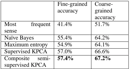
Table 4: The semi-supervised KPCA model outperforms supervised na¨ıve Bayes and maximum entropy models, as well as the most-frequent-sense and supervised KPCA baseline models.
Fine-grained accuracy
Coarse-grained accuracy Most frequent
sense
41.4% 51.7%
Na¨ıve Bayes 55.4% 64.2%
Maximum entropy 54.9% 64.1% Supervised KPCA 57.0% 66.6% Composite
semi-supervised KPCA
57.4% 67.2%
For each target word, training and test instances manu-ally tagged with WordNet senses are available. There are an average of about 10.5 senses per target word, rang-ing from 4 to 19. All our models are evaluated on the Senseval-2 test data, but trained on different training sets. We report accuracy, the number of correct predictions over the total number of test instances, at two different levels of sense granularity.
The supervised models are trained on the Senseval-2 training data. On average, 137 annotated training in-stances per target word are available.
In addition to the small annotated Senseval-2 data set, the semi-supervised KPCA model can make use of large amounts of unannotated data. Since most of the Senseval-2 verb data comes from the Wall Street Journal, we choose to augment the Senseval-2 data by collecting additional training instances from the Wall Street Jour-nal Tipster corpus. In order to minimize the noise during KPCA learning, we only extract the sentences in which the target word occurs. For each target word, up to 1500 additional training instances were extracted. The result-ing trainresult-ing corpus for the semi-supervised KPCA model is more than 10 times larger than the Senseval-2 training set, with an average of 1637 training instances per target word.
The set of features used is as described by Yarowsky and Florian (2002) in their “feature-enhanced na¨ıve Bayes model”, with position-sensitive, syntactic, and lo-cal collocational features.
6
Results
Table 5: Semi-supervised KPCA is not necessary when supervised KPCA is very confident.
Fine-grained accuracy
Coarse-grained accuracy
Supervised KPCA 62.1% 71.3%
Semi-supervised KPCA
57.1% 67.1%
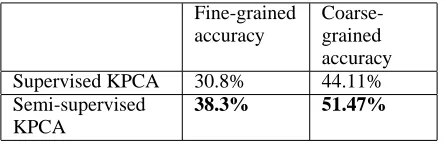
Table 6: Semi-supervised KPCA outperforms supervised KPCA when supervised KPCA is not confident: adding training data helps when there are no similar instances in the training set. Supervised KPCA 30.8% 44.11% Semi-supervised
KPCA
38.3% 51.47%
accuracy of the supervised KPCA model.
Overall, with the addition of the semi-supervised model, the accuracy for disambiguating the verbs in-creases from 57% to 57.4% on the fine-grained task, and from 66.6% to 67.2% on the coarse-grained task.
In our composite model, the supervised KPCA model predicts senses with high confidence for more than 94% of the test instances. The predictions of the semi-supervised model are used for the remaining 6% of the test instances. Table 5 shows that it is not necessary to use the semi-supervised training model for all the train-ing instances. In fact, when the supervised model is con-fident, its predictions are significantly more accurate than those of the semi-supervised model alone.
When the predictions of the supervised KPCA model are not accurate, the semi-supervised KPCA model out-performs the supervised model. This happens when (1) there is no training instance that is very similar to the test instance considered and when (2) in the absence of rele-vant features to learn from in the small annotated train-ing set, the supervised KPCA model can only predict the most frequent sense for the current target. In these condi-tions, our experiment results in Table 6 confirm that the semi-supervised KPCA model benefits from the large ad-ditional training data, suggesting it is able to learn useful feature conjunctions, which help to give better predic-tions.
The composite semi-supervised KPCA model there-fore chooses the best model depending on the degree of confidence of the supervised model. All the KPCA weights, for both the supervised and the semi-supervised model, have been pre-computed during training, and it is therefore inexpensive to switch from one model to the other at testing time.
7
Conclusion
We have proposed a new composite semi-supervised WSD model based on the Kernel PCA technique, that employs both supervised and semi-supervised compo-nents. This strategy allows us to combine large amounts of cheap unlabeled data with smaller amounts of labeled data. Experiments on the hard-to-disambiguate verbs from the Senseval-2 English lexical sample task confirm that when the supervised KPCA model is insufficiently confident in its sense predictions, taking advantage of the semi-supervised KPCA model trained with the unlabeled data can help to give a better prediction. The composite semi-supervised KPCA model exploits this to improve upon the accuracy of the supervised KPCA model intro-duced by Wu et al. (2004).
References
Martin Chodorow, Claudia Leacock, and George A. Miller. A topical/local clas-sifier for word sense identification. Computers and the Humanities, 34(1-2):115–120, 1999. Special issue on SENSEVAL.
Hoa Trang Dang and Martha Palmer. Combining contextual features for word sense disambiguation. In Proceedings of the SIGLEX/SENSEVAL Workshop on Word Sense Disambiguation: Recent Successes and Future Directions, pages 88–94, Philadelphia, July 2002. SIGLEX, Association for Computa-tional Linguistics.
Konstantinos I. Diamantaras and Sun Yuan Kung. Principal Component Neural Networks. Wiley, New York, 1996.
Adam Kilgarriff and Joseph Rosenzweig. Framework and results for English Senseval. Computers and the Humanities, 34(1):15–48, 1999. Special issue on SENSEVAL.
Adam Kilgarriff. English lexical sample task description. In Proceedings of Senseval-2, Second International Workshop on Evaluating Word Sense Dis-ambiguation Systems, pages 17–20, Toulouse, France, July 2001. SIGLEX, Association for Computational Linguistics.
Dan Klein and Christopher D. Manning. Conditional structure versus conditional estimation in NLP models. In Proceedings of EMNLP-2002, Conference on Empirical Methods in Natural Language Processing, pages 9–16, Philadel-phia, July 2002. SIGDAT, Association for Computational Linguistics.
Taku Kudo and Yuji Matsumoto. Fast methods for kernel-based text analysis. In Proceedings of the 41set Annual Meeting of the Asoociation for Computa-tional Linguistics, pages 24–31, 2003.
S. Mika, B. Sch¨olkopf, A. Smola, K.-R. M¨uller, M. Scholz, and G. R¨atsch. Ker-nel PCA and de-noising in feature spaces. Advances in Neural Information Processing Systems, 1999.
Raymond J. Mooney. Comparative experiments on disambiguating word senses: An illustration of the role of bias in machine learning. In Proceedings of the Conference on Empirical Methods in Natural Language Processing, Philadel-phia, May 1996. SIGDAT, Association for Computational Linguistics.
Martha Palmer, Christiane Fellbaum, Scott Cotton, Lauren Delfs, and Hoa Trang Dang. English tasks: All-words and verb lexical sample. In Proceedings of Senseval-2, Second International Workshop on Evaluating Word Sense Dis-ambiguation Systems, pages 21–24, Toulouse, France, July 2001. SIGLEX, Association for Computational Linguistics.
Ted Pedersen. Machine learning with lexical features: The Duluth approach to SENSEVAL-2. In Proceedings of Senseval-2, Second International Work-shop on Evaluating Word Sense Disambiguation Systems, pages 139–142, Toulouse, France, July 2001. SIGLEX, Association for Computational Lin-guistics.
Bernhard Sch¨olkopf, Alexander Smola, and Klaus-Rober M¨uller. Nonlinear com-ponent analysis as a kernel eigenvalue problem. Neural Computation, 10(5), 1998.
C. J. Twining and C. J. Taylor. Kernel principal component analysis and the con-struction of non-linear active shape models. In Proceedings of BMVC20001, 2001.
Dekai Wu, Weifeng Su, and Marine Carpuat. A Kernel PCA method for superior word sense disambiguation. In Proceedings of the 42nd Annual Meeting of the Association for Computational Linguistics, Barcelona, July 2004.