cloud cavitation
with application to burst wave lithotripsy
Thesis by
Kazuki Maeda
In Partial Fulfillment of the Requirements for the Degree of
Doctor of Philosophy
CALIFORNIA INSTITUTE OF TECHNOLOGY Pasadena, California
2018
© 2018 Kazuki Maeda
ACKNOWLEDGEMENTS
First and foremost, I truly thank my advisor Tim Colonius for his continuous support throughout the thesis project. I would not have completed this thesis not for his patience and trust in my work. I have learned from Tim not only computational fluid dynamics, but also various skills and techniques to run and manage scientific research projects, all of which are valuable in my continuing career. I thank John Brady, Guillaume Blanquart, and Michael Shapiro for serving as thesis committee members and providing valuable suggestions and comments on the thesis.
I acknowledge the members of the PPG research project for collaborations and for providing valuable suggestions on my work at the semi-annual project meetings and other occasions. I especially thank Adam Maxwell, Wayne Kreider, and Michael Bailey in the Applied Physics Laboratory at University of Washington for hosting my visits to conduct laboratory experiments.
I thank Daniel Fuster for hosting my visit to the Institut Jean Le Rond D’Alembert at Pierre and Marie Curie University.
I cannot thank too much the past and present fellow students of the computational flow physics group, including Vedran Coralic, Sebastian Liska, Jomela Meng, Aaron Towne, Chen Tsai, Jeesoon Choi, Andres Goza, Phillipe Tosi, Andre da Silva, Marcus Lee, Ke Yu, and Ethan Pickering for countless discussions. I acknowledge Jean-Christophe Veilleux and Mathis Bode for research collaborations. I also thank all other members of the group and the multiphase flow research meeting, including Gerry Della Rocca, Oliver Schmidt, Georgious Rigas, Gianmarco Mengaldo, Kevin Schmidtmier, and Erick Salcedo.
Finally, I truly thank my wife Nadia, our son Eugene and all our family members for their continuous support and encouragement.
Modeling, numerical simulations, and experiments are used to investigate the dy-namics of cavitation bubble clouds induced by strong ultrasound waves.
A major application of this work is burst wave lithotripsy (BWL), recently proposed method of lithotripsy that uses pulses (typically 10 wavelengths each) of high-intensity, focused ultrasound at a frequency of O(100) kHz and an amplitude of O(1) MPa to break kidney stones. BWL is an alternative to standard shockwave lithotripsy (SWL), which uses much higher amplitude shock waves delivered at a typically much lower rate. In both SWL and BWL, the tensile component of the pressure can nucleate cavitation bubbles in the human body. For SWL, cavitation is a significant mechanism in stone communition, but also causes tissue injury. By contrast, little is yet known about cavitation in BWL.
To investigate cloud cavitation in BWL, two numerical tools are developed: a model of ultrasound generation from a medical transducer, and a method of simulating clouds of cavitation bubbles in the focal region of the ultrasound. The numerical tools enable simulation of the cavitation growth and collapse of individual bub-bles, their mutual interactions, and the resulting bubble-scattered acoustics. The numerics are implemented in a massively parallel framework to enable large-scale, three-dimensional simulations. Next, the numerical tools are applied to bubble clouds associated with BWL. Additionally, laboratory experiments are conducted
Maeda, K. and T. Colonius. “Bubble cloud dynamics in an ultrasound field”. In:
arXiv:1805.00129.
K.M conducted simulation and experiment, prepared the data, and wrote the manuscript.
Maeda, K., A.D. Maxwell, W. Kreider, T. Colonius, and M.R. Bailey. “Quantification of the energy shielding of kidney stones by cavitation bubble clouds during Burst Wave Lithotripsy”. In:In preparation.
K.M conducted modeling, simulation, and experiment, prepared the data, and wrote the manuscript.
Bode, M., S. Satcunanathan, K. Maeda, T. Colonius, and H. Pitsch (2018). “An equation-of-state tabulation approach for injectors with non-condensable gases: Development and analysis”. In:The 10th International Symposium on Cavitation
(CAV2018).
K.M conceptualized the numerical model and helped prepare the manuscript. Maeda, K. and T. Colonius (2018a). “Eulerian-Lagrangian method for simulation
of cloud cavitation”. In:Journal of Computational Physics. doi: http://doi. org/10.1016/j.jcp.2018.05.029.
K.M conducted modeling, simulation and experiment, prepared the data, and wrote the manuscript.
– (2018b). “Numerical simulation of the bubble cloud dynamics in an ultrasound field”. In:The 10th International Symposium on Cavitation (CAV2018).
K.M conducted simulation, prepared the data, and wrote the manuscript.
Maeda, K., Kreider, A.D. W. Maxwell, T. Colonius, and M.R. Bailey (2018). “Com-bined numerical and experimental analysis of cloud cavitation for burst wave lithotripsy”. In:The ASME 5th Joint US-European Fluids Engineering Summer
Conference (FEDSM2018).
K.M conducted modeling, simulation, and experiment, prepared the data, and wrote the manuscript.
Maeda, K., A.D. Maxwell, W. Kreider, T. Colonius, and M.R. Bailey (2018). “In-vestigation of the energy shielding of kidney stones by cavitation bubble clouds during burst wave lithotripsy”. In:The 10th International Symposium on
Cavita-tion (CAV2018).
K.M conducted modeling, simulation, and experiment, prepared the data, and wrote the manuscript.
Society of America. Vol. 143. 3. ASA, pp. 1861–1861. doi:https://doi.org/ 10.1121/1.5036106.
K.M conducted numerical simulation.
Veilleux, J-C., K. Maeda, T. Colonius, and J.E. Shephered (2018). “Transient cavi-tation in pre-filled syringes during autoinjector actuation”. In:The 10th
Interna-tional Symposium on Cavitation (CAV2018).
K.M provided the numerical setup and helped preparing the manuscript.
Maeda, K. and T. Colonius (2017). “A Source Term Approach for Generation of One-way Acoustic Waves in the Euler and Navier-Stokes equations”. In:Wave Motion 75, pp. 36–49. doi:http://doi.org/10.1016/j.wavemoti.2017.08.004. K.M conducted modeling and simulation, prepared the data, and wrote the manuscript.
Maeda, K., T. Colonius, W. Kreider, A. D. Maxwell, and M. Bailey (2017). “Quan-tification of the shielding of kidney stones by bubble clouds during burst wave lithotripsy”. In:Journal of the Acoustical Society of America. Vol. 141. 5. ASA, pp. 3673–3673. doi:http://doi.org/10.1121/1.4987968.
K.M conducted modeling, simulation and experiment, prepared the data, and wrote the manuscript.
Maeda, K., T. Colonius, W. Kreider, A. Maxwell, and M. Bailey (2016). “Modeling and experimental analysis of acoustic cavitation bubble clouds for burst-wave lithotripsy”. In:Journal of the Acoustical Society of America. Vol. 140, pp. 3307– 3307. doi:http://doi.org/10.1121/1.4970532.
K.M conducted modeling, simulation, and experiment, prepared the data, and wrote the manuscript.
Maeda, K., W. Kreider, A. Maxwell, B. Cunitz, T. Colonius, and M. Bailey (2015). “Modeling and experimental analysis of acoustic cavitation bubbles for Burst Wave Lithotripsy”. In:Journal of Physics: Conference Series656.1, p. 012027. doi:http://doi.org/10.1088/1742-6596/656/1/012027.
Acknowledgements . . . iii
Abstract . . . iv
Published Content and Contributions . . . vi
Table of Contents . . . viii
List of Illustrations . . . x
List of Tables . . . xiii
Nomenclature . . . xiv
Chapter I: Introduction . . . 1
1.1 Cloud cavitation in lithotripsy - historical perspective . . . 1
1.2 Burst wave lithtoripsy . . . 2
1.3 Method of modeling the dynamics of cloud cavitation . . . 3
1.4 Numerical approaches . . . 6
1.5 Motivation and objectives . . . 9
1.6 Summary of contributions . . . 10
1.7 Organization of this thesis . . . 11
Chapter II: An one-way acoustic source model for simulation of medical ultrasound . . . 13
2.1 Overview . . . 13
2.2 Model . . . 14
2.3 Numerical implementation . . . 21
2.4 Numerical Results . . . 22
2.5 Summary . . . 35
Chapter III: Eulerian-Lagrangian method for simulation of cloud cavitation . 36 3.1 Overview . . . 36
3.2 Governing equations . . . 38
3.3 Model reduction of the three-dimensional volume-averaged equations 46 3.4 Numerical results . . . 54
3.5 Summary . . . 69
3.A Numerical algorithm . . . 70
3.B Scaling and performance of the flow solver . . . 70
3.C Speedup with the reduced model . . . 72
3.D Details of the sub-grid modeling to obtainp∞for the three-dimensional model . . . 73
Chapter IV: Dynamics of bubble clouds in an ultrasound field . . . 76
4.1 Overview . . . 76
4.2 Experimental high-speed imaging . . . 80
4.3 Theory and scaling for the dynamics of bubble clouds . . . 81
4.4 Cloud cavitation in a focused ultrasound wave . . . 84
4.6 Implications for cavitation in lithotripsy . . . 100
4.7 Summary . . . 102
4.A Local cloud interaction parameter . . . 103
4.B Simulation of the bubble cloud dynamics in the long wavelength regime104 Chapter V: Quantification of the energy shielding of kidney stones by cavita-tion bubble clouds . . . 108
5.1 Overview . . . 108
5.2 Experimental setup . . . 108
5.3 Simulation setup . . . 109
5.4 Results and discussion . . . 110
5.5 Summary . . . 115
Chapter VI: Concluding remarks . . . 116
6.1 Conclusions . . . 116
6.2 Recommendations for future work . . . 118
Bibliography . . . 120
Appendix A: Note on the dynamics of spherical bubbles under mutual inter-actions . . . 128
A.1 Overview . . . 128
A.2 Rayleigh-Plesset equation extended for multiple bubbles . . . 128
A.3 Canonical formulation . . . 131
Number Page
1.1 Fragmentation of a model stone during BWLin vitro. . . 2 1.2 Comparison of representative focal waveforms of SWL and BWL . . 3 1.3 Cavitation bubble cloud observed in an experimental high-speed
imaging during a passage of focused ultrasound in water. . . 3 1.4 Schematic of an Eulerian-Lagrangian method employed by Kameda
and Matsumoto (1996). . . 6 2.1 Pressure distribution on thez-axis att =49.3 µs. . . 24 2.2 Distribution of the scaled pressure on the r-axis and magnitude of
the scaled error between the analytical and numerical solutions . . . . 26 2.3 L1,2,∞-norm of the error between the analytical solution and the
nu-merical solution att =5.12 µs. . . 27 2.4 The axial and focal scans of the pressure field in water by the SEA
hydrophone forp0 =1.0×10⁴Pa. . . 28 2.5 The focal pressure evolutions in water. . . 29 2.6 Flooded pressure contour of the simulated acoustic fields. . . 31 2.7 Multiarray transducer with 18 elements considered in the present study. 32 2.8 Scans of the pressure field around the focal point generated by the
multi-element array medical transducer. . . 33 2.9 Pressure iso-contours of the simulated acoustic fields generated by
the multi-element array medical transducer. . . 34 3.1 Schematic of the smearing of the volume of Lagrangian bubbles on
neighboring finite volume cells defined on various grids. . . 50 3.2 Schematic of the technique to estimate p0cell in the reduced models. . 51 3.3 Evolution of a single, isolated bubble. . . 56 3.4 Scattered pressure wave from a single, isolated bubble. . . 57 3.5 Schematic of the initial condition and the three-dimensional
compu-tational grid (only one of every two cells shown) for the bubble screen problem. . . 58 3.6 Evolution of the void fraction and the pressure at the origin in the
3.7 Snapshots of the pressure and the void fraction contours in the bubble screen problem. . . 60 3.8 Evolution of CTE mp/CTW and its correlation with β0 and NC in the
bubble screen problem. . . 61 3.9 Evolution of the ensemble averaged values of void fraction and the
maximum bubble radius in the bubble screen problem. . . 63 3.10 Fluctuations inINthrough 15 simulations of the bubble screen problem. 64 3.11 Schematic of the simulation setup for the wave-cloud interaction
problem. . . 65 3.12 Evolution of the void fraction during cloud-wave interaction. . . 66 3.13 Snapshots of the bubble cloud during the simulation using the
three-dimensional model. . . 67 3.14 Evolution of the void fraction and the kinetic energy of liquid induced
by the bubbles in the proximal and distal halves of the cloud. . . 68 3.15 Scaling performance of the flow solver. . . 71 3.16 The speedup performance of the solver for 5003cells. . . 71 3.17 Speed up by using the two dimensional model, with and without
modelingp0cell. . . 72 4.1 Evolution of a bubble cloud excited with a single cycle of sinusoidal
wave with a frequency of f =50 kHz. . . 78 4.2 Evolution of the radii of representative bubbles at distinct radial
coordinates in the cloud. . . 79 4.3 Schematic of the experimental setup. . . 80 4.4 Measurement of the focal pressure evolution used for calibration of
the modeled transducer in the simulation. . . 81 4.5 High-speed images showing evolution of the bubble cloud excited by
a focused ultrasound wave. . . 82 4.6 Schematic of the numerical setup. . . 84 4.7 Images of the bubble cloud obtained in the experiment and simulation. 86 4.8 Comparisons of the evolutions of the two dimensional void fraction
of bubbles during the experiment and the simulations. . . 86 4.9 Evolution of the moment of volume and that of the kinetic energy. . . 88 4.10 Evolution of the moment of volume with A=10. . . 90 4.11 Images of the bubble clouds with various values ofB0att
∗ =
5.7. . . 90 4.12 Correlations of the time averaged moment of volume of ensemble
4.14 Evolution of the moment of kinetic energy. . . 92
4.15 Evolution of the mean radius of bubbles in the cloud. . . 94
4.16 Dynamic interaction parameter plotted against the amplitude of pres-sure excitation for various values of B0. . . 94
4.17 Scattered plots of the time averaged moments of kinetic energy against B0andB. . . 95
4.18 Scattered plots of the time averaged moments of volume againstB. . 97
4.19 Evolution of the scattered pressure field at a distance r = 8Rc from ensemble averaged clouds. . . 97
4.20 Contours of the scattered pressure field and polar plots of the root-mean-square pressure. . . 98
4.21 Scatter plots of the root-mean-square pressure againstB0andB. . . . 99
4.22 Scatter plots of the moments of kinetic energy againstprms. . . 100
4.23 Contours of the maximum pressure over the course of the simulations without and with the bubble cloud. . . 101
4.24 Evolutions of the void fractions of monodisperse and polydisperse clouds. . . 104
4.25 Scatter plot of the maximum bubble radius about the initial bubble. . 105
4.26 Scattered plots of the maximum radius of each bubble with distinct values ofB0. . . 106
5.1 Schematic of the experimental setup. . . 109
5.2 Evolution of the focal pressure. . . 110
5.3 Evolution of the projected area of bubble cloud. . . 111
5.4 Images of representative bubble clouds in the experiment and the simulation. . . 111
5.5 Snapshots of the pressure contour. . . 112
5.6 Normalized contour of the imaging functional obtained from the experiment and the simulation. . . 113
LIST OF TABLES
Number Page
BWL. Burst Wave Lithotripsy.
CFD. Computational Fluid Dynamics. DNS. Direct Numerical Simulation.
ESWL. Extracorporeal ShockWave Lithotripsy.
FV-WENO. Finite Volume Weighted Essentially Non-Oscillatory Scheme. HIFU. High Intensity Focused Ultrasound.
KZK. Khokhlov-Zabolotskaya-Kuznetsov Equation. LES. Large Eddy Simulation.
C h a p t e r 1
INTRODUCTION
1.1 Cloud cavitation in lithotripsy - historical perspective
When tensile stress is applied to a liquid and the local pressure falls below the vapor pressure, clouds of bubbles are nucleated and rapidly collapse on recovery of the pressure. This phenomenon is denoted as cavitation, or cloud cavitation, and is of critical importance in various applications. Cloud cavitation occurs mainly in two scenarios: decrease in the hydrodynamic pressure in a liquid flow, typically on the surface of an immersed body, and propagation of tensile components of a pressure wave including acoustic and shockwaves. The two regimes of cavitation are heuristically distinguished as inertial (hydrodynamic)- and acoustic cavitation. The study of cloud cavitation finds its roots in industrial needs of understanding the physical process of inertial cavitation for better designing hydraulic machines (Plesset and Ellis, 1955; Acosta, 1958; Kato, 1975). Inertial cavitation has a critical impact on the performance of hydrofoils, ship propellers, turbo-machineries and pumps: continuous cavitation on a hydrofoil/propeller largely complicates the surrounding flow structures to affect the drag and lift forces/thrust; violent collapse of caviation bubble clouds results in material damage (cavitation erosion) and noise emission. A vast amount of literatures has addressed cavitation in this context since early 20th century to date (Knapp, 1954; Brennen, 2013).
Figure 1.1: Fragmentation of a model stone during BWL in vitro. The scale bar denotes 1 cm. Reprinted from Maxwell et al. (2015) with the permission of Elsevier. © 2015 by Elsevier.
a negative amplitude of O(1−10) MPa. Meanwhile, in the actual treatment, due to the high amplitude of the negative pressure, bubble clusters are nucleated in the tensile tail and then violently collapse in the human body. The collapse of the bubble clusters on/near kidney stones can enhance stone comminution by erosion, while those occurring in the surrounding tissues result in severe injuries (Coleman et al., 1987; Pishchalnikov et al., 2003; McAteer et al., 2005; Bailey et al., 2006). Precise control of the nucleation sites of bubble-clusters has remained a challenge and the injury is thought to be unavoidable, and this has been seen as a major disadvantage of ESWL.
1.2 Burst wave lithtoripsy
Burst wave lithotripsy (BWL) has been recently proposed as a noninvasive alternative to ESWL (Maxwell et al., 2015; Thoma, 2014). BWL is a HIFU-based lithotripsy that uses a sinusoidal form of a focused pressure wave, burst wave, with a peak maximum amplitude ofO(1−10)MPa and a frequency ofO(100)kHz for kidney stone comminution. Figure 1.1 shows fragmentation of a model stone using BWLin
vitro. It has been empirically found that, compared to SWL, BWL can comminute stones into smaller fragments. Figure 1.2 shows comparisons of the representative focal waveforms of ESWL and BWL. Due to the lower peak pressure than SWL, BWL expects less violent cavitation collapse and thus lower risk of potential injury. The demonstration of stone comminution was made in vitro in highly degassed water with approximately 20% O2saturation, such that cavitation was not observed. Later in water with 65% O2saturation, however,O(1)mm size of cavitation bubble clouds are identified around the focal region without stone model during a passage of the burst wave with a frequency of 335 kHz and a peak maximum amplitude of 6 MPa (Maeda, Kreider, et al., 2015).
Figure 1.2: Comparison of representative focal waveforms of (a)SWL and (b)BWL. Reprinted from Maxwell et al. (2015) with the permission of Elsevier. © 2015 by Elsevier.
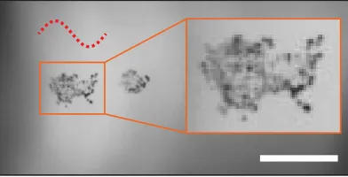
Figure 1.3: Cavitation bubble cloud observed in an experimental high-speed imaging during a passage of focused ultrasound in water. The dotted line indicates the wavelength of the burst wave. The scale bar denotes 5 mm.
importance on the safety and efficacy for clinical applications. 1.3 Method of modeling the dynamics of cloud cavitation
Although experiment provides critical insights into cloud cavitation phenomena, precise measurement of individual bubbles has been a challenging task due to the fast dynamics of bubble oscillations at the small spatial scale. Modeling and numerical simulations have been therefore central tools for quantification of the dynamics.
extended to many forms to include the effects of damping mechanisms of liquid viscosity, acoustic radiation, and heat and mass transfer (Gilmore, 1952; Plesset and Prosperetti, 1977; Keller and Miksis, 1980; Preston et al., 2007; Bergamasco and Fuster, 2017), non-spherical deformation, viscoelasticity of surrounding liquid (Church, 1995; Freund, 2008; Gaudron et al., 2015), to name but a few. The equation predicts the complex, nonlinear response of bubble oscillations under harmonic far-field pressure excitation with a large amplitude, including bifurcation and chaos, and resulting acoustic emission rich in harmonics (Lauterborn and Cramer, 1981; Prosperetti et al., 1988; Brenner et al., 2002).
A major difficulty in modeling cloud cavitation stems from multiple length-scales of the problem, ranging from the size of a bubble, inter-bubble distance, and the size of a bubble cloud, to the pressure wavelength. Existing methods of modeling can be categorized into two major approaches, both of which impose certain assumptions on separations of the scales: (1) tracking the dynamics of individual bubbles under mutual-interactions, which we denote as Lagrangian point-bubble approach1 and (2) considering the dynamics of macroscopic bubbly-mixture then modeling the averaged effect of the bubble dynamics at the small scales on the mixture without tracking individual bubbles, which we denote as the mixture-averaging approach. In the Lagrangian point-bubble approach, the Rayleigh-Plesset equation (or one of its many generalizations) is extended to a system of multiple bubbles by formulating the potential flow induced by each bubble as a monopole (or poles represented by certain set of harmonic functions that defines the bubble-shape when non-spherical deformation is considered), and expressing their interactions using a multi-pole ex-pansion (Takahira et al., 1994; Doinikov, 2004; Ilinskii et al., 2007). The dynamical equation becomes a non-autonomous, implicit, linear system of ODEs in terms of the radius and radial velocity of each bubble. The typical modeling assumption made here is that the liquid is incompressible at a scale of bubble cloud; the char-acteristic wavelength of the pressure field is much larger than the size of the cloud. The solution of an N-body problem limits to a relatively small number of bubbles
1Lagrangian point-particle approachgenerally covers wide variety of numerical methods for
(Chahine and H. Liu, 1985; Bremond et al., 2006; Zeravcic et al., 2011).
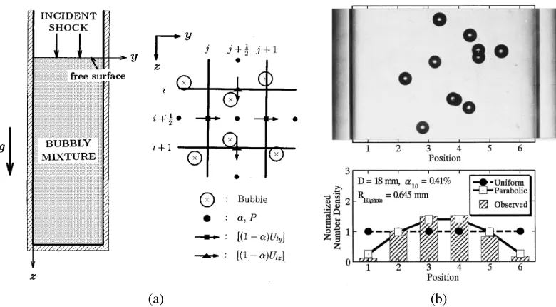
The mixture-averaging approach was pioneered by vanWijngaarden (L. vanWijn-gaarden, 1966; L vanWijnvanWijn-gaarden, 1968). In the approach, bubbly-liquid is modeled as a continuous mixture. The volume of dispersed bubbles is converted to a contin-uous void fraction field in a control volume that contains a sufficiently large number of bubbles. Here, critical modeling assumption is that the length-scale of the con-trol volume (averaging length-scale) is larger than the characteristic inter-bubble distance. The dynamics of the mixture are formulated as conservation equations about the volume-averaged mass, momentum and energy of the mixture as partial differential equations (PDEs), and they are denoted as volume-averaged equations. The volumetric change in the gas-phase is closed by considering the averaged con-tributions of the oscillations of bubbles in response to pressure fluctuations in the mixture. Bubbles are typically modeled as spherical cavities, of which dynamics are described by the Rayleigh-Plesset-type of equation. The radius and coordinate of the bubbles are treated as statistically averaged quantities in the field of mixture, rather than deterministic variables defined at each single bubble. Inter-bubble in-teractions can be modeled by an effective pressure in the mixture that forces the oscillations of bubbles, enabling the methods to avoid explicitly solving for the interactions. Caflisch et al. (1985) later showed that the volume-averaged equations formulated by vanWijngaarden can be derived by an adaptation of an ensemble-averaged equation for multiple-scattering of waves in a random media introduced by Foldy (1945). The family of volume- and ensemble-averaged equations is gen-erally denoted as mixture-averaged equations, and has been applied to great many problems including acoustic/shock propagation in bubbly liquid and other regimes of bubbly flows.
(a) (b)
Figure 1.4: Schematic of an Eulerian-Lagrangian method employed by Kameda and Matsumoto (1996). Reprinted from Kameda and Matsumoto (1996) with the permission of AIP Publishing. © 1996 by AIP Publishing.
be modeled by existing methods of simulation with reasonable accuracy, and the effects of cloud cavitation in HIFU have thus been elusive.
1.4 Numerical approaches
Eulerian-Lagrangian method
With the growth in computational power, various numerical methods have been de-veloped to solve the mixture-averaged equations at fine spatial scales. An Eulerian-Lagrangian method has been explored as one of such methods.
bubbles on the shock propagation as well as mimicking the experimental condition of bubbles in simulation, shown in figure 1.4 (b), such that direct comparisons can be made. Those were not possible with one-dimensional classical mixture-averaging approaches that assume statistical, spatial homogeneity of the bubble distribution in the span-wise (pipe-normal) direction. The capabilities of the method are also beneficial for combined numerical and experimental analysis of cloud cavitation as demonstrated in Chapter 4 and 5.
Subgrid modeling
An important property of numerical methods of CFD is grid convergence of so-lutions, meaning that numerical solutions converge to analytical soso-lutions, if they exist, with a refinement of temporal and spatial discretization. This property is, for instance, important for Large-Eddy-Simulation (LES); the solution of LES with proper sub-grid modeling of turbulent eddies predicts the correct turbulent statis-tics without explicitly resolving the eddies, while it recovers the solution of direct numerical simulation (DNS) with grid refinement (Leonard, 1975; Meneveau and Katz, 2000).
wave that could not support pressure waves with a strong amplitude in a practical range of cloud cavitation considered in BWL. Nevertheless, the Eulerian-Lagrangian method can be potentially extended for three-dimensional problems and generalized to support strong pressure waves by combining with an appropriate background flow solver that can support strong, nonlinear pressure waves. Such extension and generalization of the method may enable accurate computation of cloud cavitation in HIFU.
Finite volume WENO scheme
modeling. This is the focus of Chapter 3. 1.5 Motivation and objectives
The motivation for the present thesis is the realization that the state-of-the-art tech-niques of CFD may further advance the existing framework of modeling the bubble cloud dynamics, and combined numerical and experimental analysis using the ad-vanced model may provide detailed insights into the dynamics of cavitation bubble clouds in an ultrasound field and enable quantification of the potential effects of cavitation on outcomes of BWL.
The overall objective of the present thesis is three-fold. The first is to develop numerical tools for simulation of cloud cavitation in intense ultrasound fields. The second is to use the tools to investigate and gain the knowledge on the bubble cloud dynamics for understanding the dynamics of bubble clouds in combination with laboratory experiment. The third is to apply the numerical tools and the knowledge to quantify the effects of cavitation on the outcomes of BWL.
1.6 Summary of contributions
In this section the contributions of the thesis that meet the objectives are summarized. • A mathematical model of an acoustic source is developed that can generate uni-directional (one-way) pressure waves from an arbitrary surface immersed in a three-dimensional computational domain. The model is implemented in the Euler equation. FV-WENO is used to simulate generation of focused ultrasound by piezo-ceramic medial transducers. Results were validated by comparing with experimental measurements (Chapter 2).
• A numerical method is developed for simulation of cloud cavitation excited by a strong ultrasound wave. It is an Eulerian-Lagrangian method with a subgrid model and a FV-WENO scheme, and implemented in a massively parallel framework for simulations of three-dimensional problems. Reduced models are introduced for simulation of bubble clouds that possess translational or axi-symmetry. The reduced model averages the Eulerian field in the direction of symmetry to reduce the total number of grid cells fromO(N3) toO(N2), whereNis the number of grid per dimension. The missing component of the pressure in the direction of symmetry is modeled as a stochastic noise at a sub-grid scale. The method is verified using problems of acoustic cavitation of a single bubble, bubble screen, and a bubble cloud. An anisotropic structure is newly identified in the bubble cloud during the passage of a focused ultrasound wave, in that proximal bubbles grow to larger radius than the distal bubbles. (Chapter 3).
energy of liquid induced by bubbles becomes larger in the proximal side of the cloud than in the distal side, with the increase of the parameter. Under pressure excitation with a high amplitude, the proximal, energetic bubbles can be locally cavitated, and this results in the anisotropic structure. Moreover, it is shown that the amplitude of the far-field, bubble-scattered acoustics is likewise scaled by the proposed parameter, and thus is correlated with the energy-localization in the cloud. The numerical results indicated that bubble clouds scatter a large portion of incoming ultrasound waves, implying that cloud cavitation cause energy shielding of nearby kidney stones. (Chapter 4). • The magnitude of the energy shielding of a kidney stone by a layer of bubble clouds nucleated on the surface of a stone model are quantified through a combined experimental and numerical study. In the experiment, bubble-scattered acoustics are measured, and the evolution of bubbles are captured by high-speed imaging. Results of the simulation show favorable agreement with the experimental measurements of bubble-scattered acoustics and high-speed imaging of bubbles. The numerical results show that up to 90% of the incoming wave energy can be scattered by the bubbles. This indicates potential loss of efficacy of the treatment due to cavitation. A strong correlation between the amplitude of the scattered acoustics and the energy shielding is discovered (Chapter 5).
• The solution method for the dynamical equation that formulates the dynamics of spherical gas bubbles under mutual interactions used in the Lagrangian point-bubble approach is discussed (Appendix A).
1.7 Organization of this thesis
In Chapters 2, the acoustic source model is developed and implemented in the Euler equation. Focused ultrasound waves generated from medical transducers are simulated using the model. Experimental validation is presented.
Chapter 3 is devoted to development of the Eulerian-Lagrangian method. Special emphasis is placed upon sub-grid models for accurate simulation of bubble dynamics and upon reduced order models for accelerate computation. Supplemental materials on the speed-up of the simulation due to the model reduction and on the sub-grid model are documented in the chapter appendixes.
devel-the long wavelength regime are documented in devel-the chapter appendix.
Chapter 5 presents quantification of the energy shielding of a model stone by a layer of cavitation bubbles during BWL through a combined experimental and numerical study.
A summary of conclusions and recommendations for future work are stated in Chapter 6.
C h a p t e r 2
AN ONE-WAY ACOUSTIC SOURCE MODEL FOR
SIMULATION OF MEDICAL ULTRASOUND
A part of this chapter is published in Wave Motion, 2017.
2.1 Overview
In this chapter, a model of an acoustic source is developed to simulate the generation of focused ultrasound by piezo-ceramic medical transducers. This aim is generalized as a mathematical problem to derive a unique, uniform distribution of source terms of the Euler- and Navier-Stokes equations on an arbitrary surface immersed in three-dimensional space to generate uni-directional (one-way) waves that propagate toward one side of the surface.
distribute singular sources of mass, momentum, and energy on a three-dimensional surface and use a smeared Dirac delta function to regularize the singular distribution to a volume surrounding the surface. The Green’s function solution for locally planar waves is then used to construct an anti-sound source for waves propagating in one direction. The superposition of these sources gives the desired one-way source. The model is validated with analytical solutions for spherical and planar waves, and then used to model a single element, high-intensity focused ultrasound (HIFU) transducer and a multi-element array medical transducer on a portion of a spherical surface. We compare the acoustic field produced by the one-way source for the single-element transducer with experimental measurements reported by Canney et al. (2008) in both linear and nonlinear regimes, and that of the multi-element array medical transducer with measurements reported by Maxell (2016) in a linear regime. The proposed model can in principle be combined with any discretization of the Euler or Navier-Stokes equations.
2.2 Model
Inhomogeneous Euler equations
To model acoustic generation in a fluid by forcing, we consider the compressible, inhomogeneous Euler equations,
∂ρ
∂t +∇ · (ρu)=S1, (2.1)
∂(ρu)
∂t +∇ · (ρuu+pI)=S2, (2.2)
∂E
∂t +∇ · [(E +p)u]=S3, (2.3) where S1, S2 and S3 represent scalar mass, vector momentum, and scalar energy sources, respectively. We close the equation by stiffened gas equation of state:
p=(γ−1)ρε−γπ∞, (2.4)
study we use (γ, π∞) = (1.4,0) for air and (γ, π∞) = (7.1,3.06× 109) for water, respectively.
Our goal is to find a combination of S1, S2 and S3 that generates one-way waves. To this aim, in the following we will compute general solutions of the equation in terms of arbitrary S1, S2 and S3. First we rewrite the equation in terms of linear perturbation about a quiescent state:
∂ρ0
∂t +ρ0∇ ·u
0=
S1, (2.5)
∂u0
∂t + 1
ρ0∇p
0= S2
ρ0, (2.6)
∂p0
∂t +γ(p0+π∞)∇ ·u
0=(γ−
1)S3, (2.7)
where scripts()0and()0denote variables at perturbed and stationary states, respec-tively. The linearized equations may be further manipulated to obtain
1 c2
0
∂2p0
∂t2 − ∇
2p0= ∂S1
∂t − ∇ ·S2, (2.8)
∂ω0
∂t =
∇ ×S2
ρ0 , (2.9)
ρ0T0∂s
0
∂t =S3− c2
0
γ−1S1, (2.10)
whereω0= ∇ ×u0is the vorticity perturbation,s0is the entropy perturbation andT0 is the backgrounds temperature. In general, with a presence of entropy source at the source surface (e.g. heat injection), the right hand side of equation (2.10) is non-zero. In the present study, to avoid generating entropy at the surface, we therefore set S3 = c20/(γ − 1)S1. The curl of the source distribution S2 will, unavoidably, create vorticity perturbations near an arbitrarily shaped surface. For some simple geometries, including plane waves, the curl will be identically zero, but, in any case, the vorticity generated will remain confined to a small Stokes layer near the surface in an otherwise quiescent media.
Using a Green’s function, the solution of the equation (2.8) is given as
p(x,t)=
∫ t
0 dτ
∫ ∞
−∞
dζG(t, τ,x,τ)(∂S1
produces the desired one-way wave field. To motivate the general case, we first examine planar, spherical, and cylindrical surfaces in the next two sections.
Plane wave
Forcing a three-dimensional, initially quiescent, unbounded field of domain is con-sidered using the source model for one-way plane wave. To this end we define a source plane represented by x = x0 on which the source of the same strength is uniformly distributed. The source termsS1andS2can be expressed as
S1=f(t)δ(x−x0) (2.12) S2=g(t)δ(x−x0), (2.13) where f(t) and g(t) are arbitrary functions satisfying causality condition: f(t) =
g(t) = 0 fort < 0. Though the analytical expressions for S1 and S2 are presented by Williams (1984), in the context of anti-sound generation for active noise control, we repeat the derivation for clarity.
The Green’s function for the one-dimensional wave equation is
G(t, τ,x,τ)= H(c(t−τ) − |x−ζ|), (2.14) whereHis Heaviside step function. SubstitutingS1andS2into the solution above, we obtain
p(x,t)=c 2
∫ t
0 dτ
∫ ∞
−∞
dζH(c(t−τ) − |ζ −x|)(∂S1
∂t − ∇ ·S2) (2.15)
=c
2
∫ t
0 dτ
∫ ∞
−∞
dζH(c(t−τ) − |ζ −x|)( Ûf(τ)δ(ζ− x0) −g(τ)δ0(ζ −x0))
(2.16)
=c
2
∫ t
0
dτH(c(t−τ) − |x0− x|) Ûf(τ)
| {z }
(A)
(2.17)
− c 2
∫ t
0 dτ
∫ ∞
−∞
dζH(c(t−τ) − |ζ−x|)g(τ)δ0(ζ −x0)
| {z }
(B)
We can compute the integrals(A)and(B)as (A)=hH(c(t−τ) − |x0−x|)f(τ)i
t
0+
∫ ∞
−∞
c(δ(c(t−τ) − |x0−x|))f(τ) (2.19)
=f(t− |x0− x|
c ) (2.20)
(B)=−
∫ t
0 dτ
∫ ∞
−∞
dζ ∂
∂ζ[H(c(t−τ) − |ζ−x|)]g(τ)δ(ζ−x0) (2.21)
=∫ t
0 dτ
∫ ∞
−∞
dζ∂|ζ−x|
∂ζ δ(c(t−τ) − |ζ −x|)g(τ)δ(ζ −x0) (2.22)
= ∫ t 0 dτ ∫ ∞ −∞
dζsgn(ζ− x)δ(c(t−τ) − |ζ −x|)g(τ)δ(ζ −x0) (2.23)
=∫ t
0
dτsgn(x0−x)δ(c(t−τ) − |x0−x|)g(τ) (2.24)
=1
cg(t−
|x0− x|
c )sgn(x0− x) (2.25)
=− 1 cg(t−
|x0−x|
c )sgn(x− x0) (2.26)
to obtain
p(x,t)= 1 2
c f(t− |x0−x|
c )+g(t−
|x0− x|
c )sgn(x−x0)
. (2.27)
Thus we see that the mass source S1 acts as a monopole that generates outgoing waves of the same amplitude and the same sign, propagating in both±x directions, while the momentum sourceS2acts as a dipole that generates outgoing waves of the same amplitude, but opposite sign, propagating in±xdirections.
By defining f(t)=g(t)/c, we obtain p(x,t)=1
2
g(t− |x0− x|
c )+g(t−
|x0−x|
c )sgn(x− x0)
(2.28)
=1
2
(1+sgn(x− x0))g(t− |x0−x| c )
(2.29)
=H(x− x0)g(t− |x−x0|
c ). (2.30)
one-way spherical wave. The wave equation in terms of xbecomes 1
c2 0
∂2p
∂t2 − (
∂2p
∂x2 + 2 x
∂p
∂x)=
∂S1
∂t − ∇ ·S2, (2.31)
where we have used the definition of Laplacian in spherical polar coordinates∇2(·)= 1
x2
∂2
∂x2x
2(·). Notice that we can reformulate the equation in terms ofx p: 1
c2 0
∂2(x p)
∂t2 −
∂2(x p)
∂r2 = x
∂
S1
∂t − ∇ ·S2
. (2.32)
Then we can apply the same Green’s function used for the plane source distribution to obtain:
x p(x,t)=c 2 ∫ t 0 dτ ∫ ∞ −∞
dζH(c(t−τ) − |ζ−x|)ζ(∂S1
∂t − ∇ ·S2) (2.33)
=c 2 ∫ t 0 dτ ∫ ∞ −∞
dζH(c(t−τ) − |ζ−x|) (2.34)
ζ[ Ûf(τ)δ(ζ −x0) −g(τ) 1
ζ2
∂
∂ζ(ζ2δ(ζ− x0))] (2.35)
=cx0 2
∫ t
0
dτH(c(t−τ) − |x0−x|) Ûf(τ)
| {z }
(A) (2.36) − cx 2 0 2 ∫ t 0 dτ ∫ ∞ −∞
dζ1
ζH(c(t−τ) − |ζ −x|)g(τ)δ
0(ζ−
x0)
| {z }
(C)
Integral(A) follows that used in the plane wave solution. The integral(C)differs from(B). We further compute
(C)=−
∫ t
0 dτ
∫ ∞
−∞
dζ ∂
∂ζ
1
ζH(c(t−τ) − |ζ −x|)
g(τ)δ(ζ− x0) (2.38)
=− ∫ t 0 dτ ∫ ∞ −∞ dζ
− sgn(ζ −x)
ζ δ(c(t−τ) − |ζ−x|) (2.39)
− 1
ζ2H(c(t−τ) − |ζ− x|)
g(τ)δ(ζ−x0) (2.40)
= 1
x0
∫ t
0
dτsgn(x0−x)δ(c(t−τ) − |x0−x|)g(τ)
| {z }
(B) (2.41) + 1 x2 0 ∫ t 0
dτH(c(t−τ) − |x0− x|)g(τ)
| {z }
(D)
. (2.42)
Integral(D)becomes (D)=
H(c(t−τ) − |x0−x|)(Gg(τ)+C) t
0
+∫ t
0
dτcδ(c(t−τ) − |x0−x|)(Gg(τ)+C(x)) (2.43)
=Gg(t−
|x0−x|
c )+C(x), (2.44)
whereGg(t)is the anti-derivative ofg(t)andC(x)is an integration constant. By using the expressions for(A) − (C), we obtain the following solution:
p(x,t)= 1 2
x0 x
c f(t− |x0−x|
c )+g(t −
|x0−x|
c )sgn(x0−x) − c
x0(Gg(t−
|x0− x|
c )+C(x))
. (2.45) C(x)can be obtained by comparing this solution with the initial condition,p(x,t = 0).
We see that, the waves generated by the mass sourceS1is a monopole solution like in the plane solution, while the waves generated by the momentum source S2 also contain a monopole solution, in addition to the dipole component seen in the plane wave solution. The monopole component induced byS2clearly originates from the spherical geometry. It is straightforward that defining
f(t)= 1 cg(t)+
1
x0(Gg(t−
|x0−x|
Despite its simplicity, this form of the one-way spherical wave source has not, to our knowledge, been previously reported.
Cylindrical wave
It is widely known that the cylindrical wave equation does not have a closed form of solution. The model of one-way cylindrical source in a simple form is therefore not available, unlike the plane or spherical one-way source. Instead, we can obtain an approximate solution in a closed form by solving the following inhomogeneous wave equation in terms of
√
x p, in analogous to equation (2.32):
1 c2
0
∂2(√x p)
∂t2 −
∂2(√x p)
∂x2 =
√ x
∂
S1
∂t − ∇ ·S2
. (2.48)
This approximation is valid for a cylindrical wave with a characteristic wave length much smaller than the radius of the cylindrical source plane (Whitham, 2011). The solution of equation(2.48) is readily available using the Green’s function:
p(x,t) = 1 2 c √ x ∫ t 0 dτ ∫ ∞ −∞
dζH(c(t−τ) − |ζ −x|)pζ(∂S1
∂t − ∇ ·S2)(2.49)
= 1 2 √ x0 √ x
c f(t− |x0−x|
c )+g(t−
|x0−x|
c )sgn(x0− x) (2.50) −√c
x0(Gg(t−
|x0− x|
c )+C(x))
. (2.51)
It is straightforward that defining f(t)= 1
cg(t)+ 1 √
x0(Gg(t−
|x0− x|
c )+C(x)) (2.52) makes the following one-way wave solution:
p(x,t)= √
x0 √
x H
(x−x0)g(t− |x0− x|
c ). (2.53)
Arbitrary, smooth surfaces
2.3 Numerical implementation
In principle, the models for one-way source derived in the previous section can be used for any numerical methods that solve the Euler or Navier-Stokes equations. For good accuracy, the waves should be introduced into a region of approximately quiescent flow, and the amplitude should be limited such that the linearization, upon which the source model rests, holds. Regardless, we can simply amend the derived source terms to the original nonlinear equations. In order to demonstrate verifica-tions and validaverifica-tions of the model, in the present chapter we use a finite-volume, fifth-order WENO scheme (Titarev and E. Toro, 2004) both in cylindrical coordi-nates with an azimuthal symmetry and Cartesian coordicoordi-nates. High-order WENO scheme is particularly capable of accurately simulating discontinuous solutions, including shockwave and material interface (Coralic and Colonius, 2014).
In the following we describe a method of numerical representation of the governing equation in cylindrical coordinates with azimuthal symmetry. That in 3D Cartesian coordinates can be trivially derived in a similar manner, and thus is omitted here. We spatially discretize the forced Euler equation in the following form:
∂q
∂t +
∂f(q)
∂z +
∂g(q)
∂r = s
g(q)+ss(
q), (2.54)
where q is the vector of conservative variables, f, g are vectors of fluxes, s is the vector of source terms and the superscripts(·)g and(·)s denote the geometrical source and the acoustic source, respectively. This formulation is convenient since the variables can be discretized in 2D Cartesian coordinates (E. F. Toro, 2013). We integrate the above equation in arbitrary finite volume grid cell
Ii,j = [zi−1/2,zi+1/2] × [rj−1/2,rj+1/2], (2.55) whereiandjare the indices of the cells inz−andr−directions, andzi±1/2andrj±1/2
are the positions of cell faces. At each finite volume cell, we express the equation in the following semi-discrete form:
dqi,j
dt = 1
∆zi
[fi−1/2,j− fi+1/2,j]+
1
∆rj
[gi,j−1/2− gi,j+1/2]
+ 1
2rj
[sgi,j−
1/2+ s
g
i,j+1/2]+ s
s
i,j. (2.56)
We express the forcing term ss defined on a surfaceΓ using the following integral representation:
ss =
∫
Γ
ΩΓ(ξ,t)δ(X(ξ,t) − x)dξ, (2.57) where ξ is the coordinate defined on Γ, ΩΓ(ξ,t) is the forcing, and X(ξ,t) ∈ Γ is
the function that maps ξ to x. In z−r 2D axi-symmetric coordinates, arbitrary surface with axi-symmetric geometry can be represented by a curve L. L can be parametrized by a single scalarξ, thus we have
ss =
∫
Γ
ΩΓ(ξ,t)δ(X(ξ,t) −x)dξ, (2.58)
wheredξis the line element of L. We express the forcing at cellIi,j by
ssi,j =
K
Õ
k=1
ΩΓ(ξk,t)δh(|X(ξk,t) − xi,j|)∆ξk, (2.59)
where δh is a smeared delta function, ∆ξk is the length of kth line elements of L, and k ∈ Z : k ∈ [1,K]. Various forms of δh are available (Peskin, 2002). In the present study we employ the second-order, two-dimensional Gaussian function:
δh(h)= 1
(√2πσ)2 e−12
h2
σ2, (2.60)
whereσis the support width. Typically σ =O(∆)is taken, where∆is the charac-teristic grid size at the region of the source. The overall rate of grid convergence of the scheme is second-order in smooth regions of the field. Note that the second order accuracy of the scheme for smooth regions is due to the second-order accurate spatial discretization of the geometrical source, shown in equation (2.56), despite 5th order WENO scheme is used for reconstruction of variables at cell faces. Tem-poral integration of the partial differential equation is realized by third-order total variation diminishing Runge-Kutta scheme (TVD-RK).
2.4 Numerical Results
solutions are available. Next we consider HIFU waves produced on a portion of a spherical shell and compare with previous experimental measurements as well as numerical solutions employing the KZK equation. Finally, we apply the spherical one-way source to 3D simulation of a ultrasound generation with a multi-element array medical transducer, and then compare the simulated acoustic fields with experimental measurements.
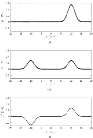
Simulation of a plane Gaussian pulse
We first simulate a one-way, Gaussian acoustic pulse in air propagating in +z direction from the source distributed on the plane ofz =0. Onz−r Cartesian grid, since the line source is aligned on theraxis, source representation can be simplified by smearing the source in±zdirection to express the source term as
ssi,j = ΩΓ(t)δh(|ri|), (2.61) whereΩΓ(t)= [f(t)/c0, f(t),0,c02f(t)/(γ −1)]and
f(t)= √pa 2πσt
e
−1 2
(t−t
0)2
σ2
t , (2.62)
where σt is the support width of the Gaussian pulse in the time space and t0 is the delay. We take pa = 10 Pa, σt = 5 µs and t0 = 20 µs. The simulation domain is z ∈ [−20,20] and r ∈ [0,20] mm. The initial condition is given by (ρ,u,p)=(1.204,0,101325), where the density, velocity, and pressure are in kg/m3, m/s and Pa, respectively. The simulation is evolved with a constant time-step,
∆t = 160 ns. 200×100 uniform computational grids are used.
-20 -15 -10 -5 0 5 10 15 20 -0.2
0 0.2 0.4 0.6
(a)
-20 -15 -10 -5 0 5 10 15 20
-0.2 0 0.2 0.4 0.6
(b)
-20 -15 -10 -5 0 5 10 15 20
-0.2 0 0.2 0.4 0.6
[image:38.612.145.449.135.586.2](c)
Simulation of a spherical sinusoidal pulse
Secondly, we simulate a one-way, sinusoidal acoustic pulse in water propagating inward from a uniform acoustic source distributed on a spherical shell with its center located at the origin, and with a radius ofr0 = 15 mm. The expressions used for the source terms are ΩΓ(ξ,t) = [f(t),gz(ξ,t),gr(ξ,t),c02f(t)/(γ −1)], where, with angular frequencyω =2πfs,
f(t)=pa
c0sin(ω(t−t0))+ pa
r0(Gg(ω(t−t0))+C), (2.63)
gz(ξ,t)=−pasin(ω(t −t0))cosξ, (2.64)
gr(ξ,t)=−pasin(ω(t −t0))sinξ. (2.65)
The spherical shell is represented as an upper hemi-circle in the z−r coordinate plane. ξ is defined as the polar angle that parametrizes the arc of the hemi-circle;
ξ ∈R: ξ ∈ [0, π]and X(ξ) =[r0cosξ,r0sinξ]. The geometrical components of the mass sourceGg(t)andC are expressed as
Gg(t)= ∫
−sin(ωτ)dτ= 1
ωcos(ωt), (2.66)
C =−Gg(0)= −ω1. (2.67)
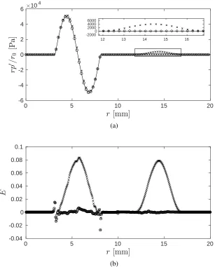
We takepa = 10 Pa, fs = 3.0×10⁵Hz, andt0= π/(2f)s. The simulation domain is z ∈ [−20,20] and r ∈ [0,20] mm. We evolve the simulation with the initial condition given by (ρ,u,p) = (1000,0,101325), where the density, velocity, and pressure are in kg/m3, ms−1and Pa, respectively. The simulation is evolved with a constant time-step,∆t =20 ns. 800×400 uniform computational grids are used. In figure 2.2 (a) we compare the distribution of the analytical and numerical solutions of the pressure scaled by the radial coordinate, r p0/r0, on the r-axis at t = 5.12
0 5 10 15 20 -6
-4 -2 0 2 4 6 10
4
12 13 14 15 16
-20000 2000 4000 6000
(a)
0 5 10 15 20
-0.04 -0.02 0 0.02 0.04 0.06 0.08 0.1
[image:40.612.143.450.142.523.2](b)
Figure 2.2: (a)The distribution of the scaled pressurer p0/r0on ther-axis att =5.12
102 103 10-4
10-3 10-2 10-1 100
[image:41.612.208.398.78.267.2](a)
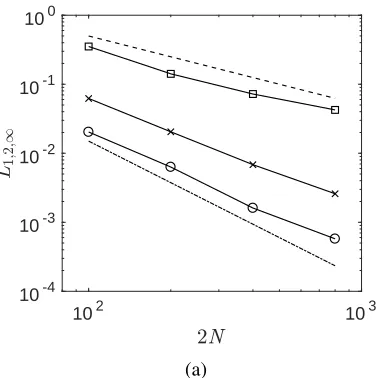
Figure 2.3: L1,2,∞-norm of the error between the analytical solution and the numeri-cal solution att =5.12µs as a function of the grid size (2N×N). Reference slopes for the first and second order convergence are included.
shows L1,2,∞-norm of the error between the analytical solution and the numerical solution withGg(t), both of which are shown in figure 2.2 (a), as a function of the grid size. The result indicates that the numerical solution is first-order accurate. While the underlying finite-volume scheme being used is second-order accurate (for smooth solution), our regularization of the singular source on the scale of the grid spacing strands a first-order error in the source representation (Tornberg and Engquist, 2003).
High-Intensity Focused Ultrasound
30 40 50 60
Axial Position [mm]
0 0.5
A
m
p
li
tu
(a)
-3 -2 -1 0 1 2 3
Transverse Position [mm] 0
0.5 1
A
m
p
li
tu
d
e
[image:42.612.166.425.79.431.2](b)
Figure 2.4: The (a)axial and (b)focal scans of the pressure field in water by the SEA hydrophone forp0= 1.0×10⁴Pa. The result of the direct numerical simulation (-), and SEA hydrophone measurement by Canney et al. (2008) (◦), and O’Neal analytic solution (- -) (O’Neil, 1949) are compared.
regions on the axis, can be explained by a non-uniform velocity distribution on the piezoceramic plate of the real transducer, which is not considered in the simulation and the analytical solution.
0 0.5 1 1.5
-4 -2 0 2 4 6 8 10 12
(a)
0 0.2 0.4 0.6 0.8 1
-20 0 20 40 60
0.15 0.2 0.25 25
30 35
[image:43.612.184.415.144.554.2](b)
Figure 2.5: The focal pressure evolutions in water with (a) pa = 1.0×10⁵and (b) pa= 2.9×10⁵. In the plot (a), the result of the direct numerical simulation (–), FOPH measurement by Canney et al. (2008) (◦), and analytical solution calculated with the KZK equation presented in Canney et al. (2008) (- -) are compared. In the plot (b), the results of the direct numerical simulation with a cell size of∆x = ∆y =12.5
µm (- -) and ∆x = ∆y = 20 µm (–) are compared with FOPH measurement and analytical solution calculated with the KZK equation.
and the experimental measurement conducted by Canney et al. The corresponding solutions of the KZK equation presented in Canney et al are also plotted. In the case withpa = 1.0×10⁵Pa, shown in figure 2.5 (a), the result of the simulation agrees very well with the measurement as well as the solution of the KZK equation. The acoustic field in the focal region is in a weekly nonlinear regime. The amplitude of the positive peak is 6 MPa, while that of the negative peak is 4 MPa. The wave form is not largely distorted from a sinusoidal form. In the case with pa =2.9×10⁵Pa, shown in figure 2.5 (b), the wave form obtained by the simulations agrees well with the measurement. The maximum pressure obtained by the simulation with coarse grids is slightly lower than that of the others, shown in the inset of figure 2.5 (b). This is due to numerical dissipation that reduces the amplitude of the sharp peak formed by nonlinear sharpening. As shown by the result of the simulation using fine grids, this dissipation can be reduced by refining the grid.
figure 2.6 shows the flooded pressure contour of the simulated acoustic fields with pa= 2.9×10⁵att = 20µs andt = 70µs. The waves generated on the source plane propagate and get focused toward the focal region. Waves propagating outward from the source plane are canceled.
Multi-element array medical transducer
Finally, we simulate a focused acoustic field generated by a medical, multi-element array medical transducer in a linear regime using the one-way spherical source, and validate the simulation with an experimental measurement. The purpose of this case is to demonstrate the feasibility of the proposed source models for applications to a non-trivial source geometry.
(a)
[image:45.612.160.470.83.398.2](b)
Figure 2.6: Flooded pressure contour of the simulated acoustic fields with pa =
2.9×10⁵at (a)t =20 µs and (b)t =70 µs. The contour level is±1 MPa
not fully axi-symmetric. Therefore we use an x-y-zCartesian coordinate system in this case of simulation. To model the element, we distribute the one-way spherical source on a ring-shaped portion of a spherical surface with a radius of 150 mm with its center located at the origin. Correspondingly, using a smeared delta function, the strength of the source is regularized onto three-dimensional grid cells neighboring the surface.
The expressions used for the source terms are
ΩΓ(ξ, η,t)= χ(X)[f(t),gx(ξ, η,t),gy(ξ, η,t),gz(ξ, η,t),c20f(t)/(γ−1)], (2.68)
(a) (b)
Figure 2.7: Multiarray transducer with 18 elements considered in the present study. (a) Real transducer. The ring-shaped piezo-ceramic elements are covered by acoustic lenses. (b) Modeled source distribution used in the simulation. The length unit used in the figure is mm. Each element is modeled as a ring-shaped source plane aligned on a spherical section with a radius of 150 mm.
f(t)=pa
c0sin(ω(t−t0))+ pa
r0(Gg(ω(t−t0))+C), (2.69)
gx(ξ, η,t)=−pasin(ω(t−t0))cosξcosη, (2.70)
gy(ξ, η,t)=−pasin(ω(t−t0))cosξsinη, (2.71)
gz(ξ, η,t)=−pasin(ω(t−t0))sinξ. (2.72)
1ξandηare defined as the polar and azimuthal angles that parametrize the spherical section;ξ, η ∈R: ξ ∈ [0, π], η∈ [−π, π], andX(ξ, η)=[r0cosξcosη,r0cosξsinη,r0sinξ].
χ is an indicator function that takes a value of 1 when Lagrangian pointX(ξ, η)is within the region of the defined ring-shaped transducer surfaces, and 0 elsewhere. Gg andCfollow equations (2.66) and (2.67), respectively.
To validate the source model, we simulate a focused acoustic field in a linear regime with 20 cycles of a sinusoidal form of pressure waves with a frequency of 340 kHz and a source amplitude of 10 Pa. The spacial configuration of the source and the resulting acoustic field are symmetric along thex-yandx-zplanes that intersect the x-axis. To reduce the computational cost, we simulate a domain ofx ∈ [−160,60],
1
Note that we setξ =[ξ, η]Tin equation (2.57). For regularization of the singular sources, we
use the second-order, three-dimensional Gaussian function:δh(h)=(√ 1 2πσ)3e
−1 2
y ∈ [0,100] and z ∈ [0,100] mm, with symmetry boundary conditions applied along the x-y and x-z planes. Non-reflecting boundary conditions are applied on the other domain boundaries. The simulation is evolved with a constant time-step,
∆t = 36.7 ns. 1320×600×600 uniform computational grids are used.
-50 0 50
Position [mm] 0 0.2 0.4 0.6 0.8 1 A m p li tu d e Simulation Measurement (a)
-10 -5 0 5 10
Position [mm] 0 0.2 0.4 0.6 0.8 1 A m p li tu d e (b)
-10 -5 0 5 10
[image:47.612.110.518.172.544.2]Position [mm] 0 0.2 0.4 0.6 0.8 1 A m p li tu d e (c)
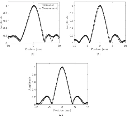
Figure 2.8: The scans of the pressure field around the focal point generated by the multi-element array medical transducer along the (a) x-axis, (b) y-axis, and (c) z-axis, respectively. The amplitudes of the pressure are normalized by their maximum values in each plot. Results obtained in the present simulation and the hydrophone measurement are compared.
Note that the linear gain of the transducer obtained from the present simulation was Ga=27.
(a) (b)
[image:48.612.129.479.181.507.2](c) (d)
Figure 2.9: Pressure iso-contours of the simulated acoustic fields with the contour levels of -200 Pa (blue color) and 200 Pa (red color) at (a)0, (b)40, (c)80 and (d)120
µs.
2.5 Summary
EULERIAN-LAGRANGIAN METHOD FOR SIMULATION OF
CLOUD CAVITATION
A part of this chapter has been accepted for publication in Journal of Computational
Physics.
3.1 Overview
In this chapter, an Eulerian-Lagrangian method is developed for simulation of cloud cavitation induced by an intense ultrasound wave.
In the method, the dynamics of bubbly-mixture is described using the volume-averaged equations of motion that fully account for the compressibility of liquid. The continuous phase is discretized on an Eulerian grid, while the gas phase is modeled as spherical, radially oscillating cavities that are tracked as Lagrangian points at the sub-grid scale. The dynamics of the continuous phase is evolved using a high-order, finite-volume weighted essentially non-oscillatory (WENO) scheme, that was originally developed for simulation of viscous, compressible, multi-component flows (Coralic and Colonius, 2014) and is capable of capturing strong pressure waves with fine structures. The volume of bubbles is mapped onto the Eulerian grids as the void fraction using a regularization kernel. The radial oscillation of each bubble is evolved by solving the Keller-Miksis equation. When the grid size is smaller than the characteristic inter-bubble distance, the method is capable of capturing the violent cavitation growth and collapse of each bubble as well as resolving the strong, complex structures of bubble-scattered pressure waves in the liquid.
of computations required to solve for the continuous phase is reduced fromO(N3) toO(N2), whereN is the number of grid cell per dimension, in comparisons to the three-dimensional model.
In order to properly close the Keller-Miksis equation, the pressure field at the sub-grid scale needs to be appropriately modeled. In the case of the three-dimensional model, in each grid cell that encloses a bubble, the contribution of the pressure wave scattered by the bubble to the averaged pressure in the cell can become significant, and thus the pressure of the cell cannot be directly used to force the oscillations of bubble. In that case, following the scheme proposed by Fuster and Colonius (2011), we obtain the component of the cell-averaged pressure that forces the oscillations of bubble by using the state of the bubble and potential flow theory at the sub-grid scale. In the two-dimensional and axi-symmetric models, the discretized pressure field is treated as uniform in the direction of symmetry, despite the three-dimensionality of the true pressure field associated with any distribution of bubbles. In order to reduce the error associated with the neglected three-dimensional pressure fluctuations, we model the spatial distribution of the pressure at the sub-grid scale as white noise. In each grid cell that contains a bubble, we estimate the variance of the noise by sampling the pressure in the neighboring cells, with an assumption that the pressure fluctuations are locally, spatially isotropic on the scale of the sampling window. The noise is expressed by superposing Fourier modes with pre-computed, randomized phases, following a method of expressing stochastic fluctuations in turbulence modeling (Bechara et al., 1994; Smirnov et al., 2001). The sub-grid closures for the three-dimensional and the reduced models are verified using the test cases of acoustic cavitation of a single bubble and a bubble screen, and a bubble cloud, respectively.
3.2 Governing equations
Volume averaged equations of motion
We introduce volume-averaged equations of motion to describe the dynamics of a mixture of dispersed bubbles and a compressible liquid in three-dimensional space. Volume-averaged equations consider the conservation of mass, momentum, and energy of the mixture as a continuum media that are defined by applying the volume averaging operator(·)to a control volume of the mixture: (·) = (1− β)(·)l +β(·)g, where β ∈ [0,1)is the volume fraction of gas (void fraction), and subscriptsl and
gdenote the liquid and gas phase, respectively. We start by writing the equations in a conservative form:
∂ρ
∂t +∇ · (ρu)= 0, (3.1)
∂(ρu)
∂t +∇ · (ρu⊗ u+pI − T)= 0, (3.2)
∂E
∂t +∇ ·
(E+p)u− T ·u
= 0, (3.3)
where ρis the density, u = (u,v,w)T is the velocity, pis the pressure and E is the total energy, respectively. Tis the effective viscous stress tensor of the mixture. We invoke two approximations widely used in averaged models at the limit of low void fraction, up to O(10−2)(Caflisch et al., 1985; Commander and Prosperetti, 1989; Fuster and Colonius, 2011). First, the density of liquid is typically much larger than that of gas, ρl ρg, and thus the density of the mixture is approximated by that of the liquid:
ρ=(1− β)ρl+ βρg ≈ (1−β)ρl. (3.4)
This approximation is clearly valid for the mixture of water and air/vapor bubbles under practical conditions. Second, the slip velocity between the two phases is zero:
With the assumption of zero slip-velocity, the momentum flux across the gas-liquid interface is effectively zero, and therefore, we approximate the total viscous stress as that in the continuous phase:
T ≈ Tl. (3.6)
Tlis the viscous stress tensor of pure Newtonian liquid:
Tl = 2µ
Dl− 1 3
(∇ ·ul)I
, (3.7)
where µl is the shear viscosity of liquid andDl is the deformation rate tensor:
Dl = 1
2
(ul+ uTl). (3.8)
In reality, spherical bubbles experience hydrodynamic forces from the surrounding liquid (Magnaudet and Legendre, 1998), and the resulting slip velocity can be non-zero. The momentum flux across the gas-liquid interface can contribute to the effective viscosity of the mixture (Zhang and Prosperetti, 1994). Such modeling is not a focus of the present study, though one could extend the present formulation to include the effect of the non-zero slip velocity on T. Nevertheless, for many practical problems of cavitation, the time scale of the radial oscillations of bubbles are estimated to be much shorter than that of the translational motions, and therefore, assumption of the zero-slip velocity is a reasonable first approximation (Caflisch et al., 1985).
Using relations (3.4-3.6), equations (3.1-3.3) can be rewritten as conservation equa-tions in terms of the mass, momentum, and energy of the liquid with source terms, as an inhomogeneous hyperbolic system:
∂ρl
∂t +∇ · (ρlul)=
ρl
1−β
∂ β
∂t + ul · ∇β
, (3.9)
∂(ρlul)
∂t +∇ · (ρlul ⊗ul+ pI − Tl)=
ρlu
1−β
∂ β
∂t + ul · ∇β
− β∇ · (pI − Tl) 1−β ,
(3.10)
∂El
∂t +∇ · ((El +p)ul− Tl·ul)= El
1−β
∂ β
∂t + ul · ∇β
− β∇ · (pul− Tl· ul)
1−β .
equations in a vector form:
∂ql
∂t +∇ · f(ql)= g(ql, β, Û
β), (3.12)
whereql = [ρl, ρlul,El]and
g= 1
1− β dβ
dt ql−
β
1−β
∇ · (f −ulql). (3.13)
For a thermodynamic closure for the liquid, we employ stiffened gas equation of state:
p=(γ−1)ρε−γπ∞, (3.14)
whereε is the internal energy of liquid, γ is the specific heat ratio, and π∞ is the stiffness, respectively. In the present study we use(γ, π∞)=(7.1,3.06108)for water, where the unit ofπ∞is Pa. At the limit of small change in the density of liquid, the equation of state can be linearized as
p= p0+c2
0(ρ− ρ0), (3.15)
where
c= pγ(p+π∞)/ρ (3.16)
is the speed of sound in liquid and the subscript 0 denotes reference states. Spatial discretization
In the following we describe a method of numerical representation of the governing equation in x − y− z 3D Cartesian coordinate. We spatially discretize equation (3.12):
∂ql
∂t +
∂fx(ql)
∂x +
∂fy(ql)
∂y +
∂fz(ql)