PARSING AND HYPERGRAPHS
Dan Klein and Christopher D. Manning
Computer Science Department
Stanford University
Stanford, CA 94305-9040
fklein, [email protected]
Abstract
While symbolic parsers can be viewed as deduction systems, this view is less natural for probabilistic parsers. We present a view of parsing as directed hypergraph analysis which naturally covers both symbolic and probabilistic parsing. We illustrate the approach by showing how a dynamic extension of Dijkstra’s algorithm can be used to construct a probabilistic chart parser with anO(n
3
)time bound for arbitrary PCFGs, while preserving as much of the
flexibility of symbolic chart parsers as allowed by the inherent ordering of probabilistic dependencies.
1
Introduction
An influential view of parsing is as a process of logical deduction, in which a parser is presented as a set of pars-ing schemata. The grammar rules are the logical axioms, and the question of whether or not a certain category can be constructed over a certain span becomes the question of whether that category can be derived over that span, treating the initial words as starting assumptions (Pereira and Warren 1983, Shieber et al. 1995, Sikkel and Nijholt 1997). But such a viewpoint is less natural when we turn to probabilistic parsers, since probabilities, or, generalizing, scores, are not an organic part of logical systems.1There is also a deep connection between logic, in particular propositional satisfiability, and directed hypergraphs (Gallo et al. 1993). In this paper, we develop and exploit the third side of this triangle, directly connecting parsing with directed hypergraph algorithms. The advantage of doing this is that scored arcsarea central and well-studied concept of graph theory, and we can exploit existing graph algorithms for probabilistic parsing. We illustrate this by developing a concrete hypergraph-based parsing algorithm, which does probabilistic Viterbi chart parsing over word lattices. Our algorithm offers the same modular flexibility with respect to exploration strategies and grammar encodings as a categorical chart parser, in the same cubic time bound, and in an improved space bound.
2
Hypergraphs and Parsing
First, we introduce directed hypergraphs, and illustrate how general-purpose hypergraph algorithms can be applied to parsing problems.
The basic idea underlying all of this work is rather simple, and is illustrated in figure 1. There is intuitively very little difference between (a) combining subtrees to form a tree, (b) combining hypotheses to form a con-clusion, and (c) visiting all tail nodes of a hyperarc before traversing to a head node. We will be building hypergraphs which encode a grammar and an input, and whose paths correspond to parses of that input.
We would like to thank participants at the 2001 Brown Conference on Stochastic and Deterministic Approaches in Vision, Language, and Cognition for comments, particularly Mark Johnson. Thanks also to the anonymous reviewers for valuable comments on the paper, and in particular for bringing Knuth (1977) to our attention. This paper is based on work supported in part by the National Science Foundation under Grant No. IIS-0085896, and by an NSF Graduate Fellowship.
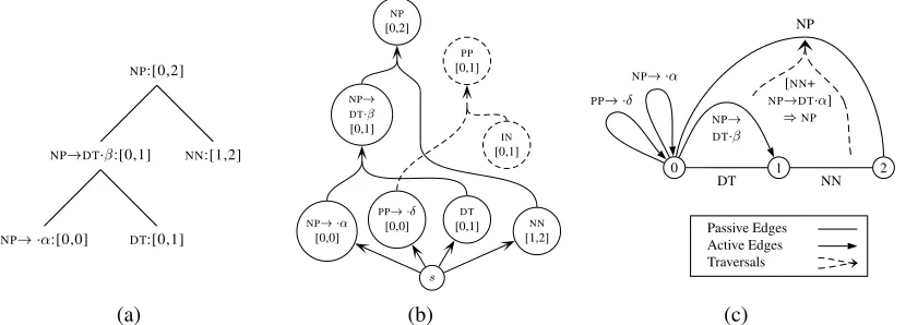
DT NN
NP DT:[0,1]
NN:[0,1]
DT:[i;k℄^NN:[k;j℄!NP:[i;j℄ NP:[0,2]
DT:[0,1]
NN:[1,2]
s NP:[0,2]
[image:2.612.115.482.133.207.2](a) (b) (c)
Figure 1: Three views of parsing: (a) tree construction, (b) logical deduction, and (c) hypergraph exploration.
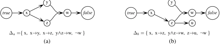
true x w false
y
z
a
=fx, x!y, x!z, y^z!w, :wg
true x w false
y
z u
b
=fx, x!z, y^z!w, z!u, :wg
(a) (b)
Figure 2: Two hypergraphs. Graph (a) is a B-path fromtruetofalse, while (b) is not. Also shown are proposi-tional rule sets to which these graphs correspond.
bis satisfiable, while
ais not.
2.1 Directed Hypergraph Basics
We give some preliminary definitions about directed hypergraphs, objects like in figure 2 , weaving in a corre-spondence to propositional satisfiability as we go. For a more detailed treatment, see (Gallo et al. 1993).
Directed hypergraphs are much like standard directed graphs. However, while standard arcs connect a single tail node to a single head node, hyperarcs connect a set of tail nodes to a set of head nodes. Often, as in the present work, multiplicity is needed only in the tail. When the head contains exactly one node, we call the hyperarc aB-arc.
Definition 1 Adirected hypergraphGis a pair(N;A)whereN is a set of nodes andAis a set of directed
hyperarcs. Adirected hyperarcis a pair(T;H)where the tailT and headHare subsets ofN.
Definition 2 AB-arcis a directed hyperarc for whichHis a singleton set. AB-graphis a directed hypergraph
where the hyperarcs are B-arcs.
It is easy to see the construction which provides the link to satisfiability. Nodes correspond to propositions, and directed hyperarcsft
1 ;:::;t
m g)fh
1 ;:::;h
n
gcorrespond to rulest 1
^^t m
!h 1
__hn. In the case of B-arcs, the corresponding rules are Horn clauses. The construction also requires two special nodes,
trueandfalse. For the Horn clause case, it turns out that satisfiability is equivalent to the non-existence of a certain kind of path fromtruetofalse.
With the notion of arc generalized, there are multiple kinds of paths. The simplest is the kind inherited from standard graphs, in which a path can enter a hyperarc at any tail node and leave from any head node.
Definition 3 A simple pathp = s ; tis a sequence(s = v 0
;a 1
;v 1
;:::a n
;v n
= t) of alternating nodes
and hyperarcs where: (1) each hyperarca
iis distinct, (2)
8i2f0;:::;n 1g;v i
2tail(a i+1
), and (3)8i2 f1;:::;ng;v
i
2head(a i
)A nodetissimply reachablefrom a nodesif a simple path exists fromstot. In the more important kind of path, each tail node must be reachable before the arc is traversable.
Definition 4 AB-pathP in a B-graphGfrom a nodesto a nodetis a minimal subgraph 2
(N P
;A P
)<G
in which: (1)s;t2N
P, and (2) 8v2N
P
fsg;9p=s;t,pa simple path inP. A nodetisB-reachable
from a nodesif a B-path exists fromstot.
This fits well with the logical rule interpretation: each hypothesis must be true before a conclusion is implied. It is perhaps not surprising, then, that B-paths fromtruetofalseare what correspond to non-satisfiability.
As an example, the B-graph in figure 2(a) is a valid B-path fromtruetofalse. However, the one in figure 2(b) is not a B-path, for two reasons. First, not all nodes are simply reachable froms(y is not). Second, even
2An important point to note is that one cannot choose only part of a hyperarc to include in a subgraph; once the arc is included, all
if we added a B-arcfxg ) y, the graph would not be minimal (the B-arcfzg ) ucould be removed). Correspondingly, there is no satisfying assignment to the rule sets in figure 2(a), whilefx=true,y=false,z=true,
w=false,u=truegis a satisfying assignment for figure 2(b).
For the remainder of this paper, we will often drop the “B-” when it is clear from context what kind of graph, arc, path, or reachability is meant.
2.2 Symbolic Parsing and Reachability
We now show how reachability in a certain hypergraph corresponds to parse existence.
In chart parsing terminology, the core declarative object is theedge, which is a labeled span. For example,
NP:[0,2] represents anNPspanning position 0 to 2. Parsing requires a grammar and an input. Here, we take the input to be alattice, which is a collection of edges stating which words can occur over which spans. The grammar is a set of context-free productions of the formC !X
1 :::X
n. These productions state that edges with labelsX
ican be combined to form an edge with label
C, subject to adjacency constraints on the edges’ spans. When a production is instantiated with specific edges, it is called atraversal. Traversals state a particular way an edge can be constructed, for example, thatS:[0,8] can be composed ofNP:[0,2] andVP:[2,8].
There is an unfortunate clash between chart parsing and hypergraph terminology. A chart (see figure 3c) is typically seen as an undirected graph with numbers as nodes and edges as arcs. Traversals, which record how an edge was constructed, are not part of the graph, but stored in an auxiliary data structure, if at all. However, in the present context, the numbers are not represented graphically (their relative structure is self-evident), edges are nodes in the hypergraph, and traversals are B-arcs in the hypergraph. For this paper, we use “edge” to refer only to labeled spans, and “arc” when we mean a (hyper)graph connection.
Given a grammarGand a latticeL, we wish to construct a hypergraph in which node reachability corre-sponds to edge parsability. This graph, which we call theinduced B-graph ofGandL, is given as follows. For each instantiation of categoryC inGas an edgeC:[i;j℄, create a node. For each instantiation of a pro-ductionC !X
1 :::X
n in
Gas a traversalC:[i;j℄!X 1:
[i;k 1
℄X 2:
[k 1
;k 2
℄ ::: X n:
[k n 1
;j℄, create a B-arc
fX1:[i;k 1
℄; X2:[k 1
;k 2
℄; :::Xn:[k n 1
;j℄g ) C:[i;j℄. This much of the construction represents the con-nectivity of the grammar. To represent the data, create a special source edges, and add arcs of the form
fsg)C:[i;j℄for each word edgeC:[i;j℄andfsg)C:[i;i℄for each categoryCwith an empty production. Similarly, we define a mappingwhich takes parse treesT to B-graphs(T), where the nodes of(T)are the edges ofT (along withs), and the B-arcs in(T)are the traversals ofT (along withsarcs to terminals inT). For example, figure 1(c) is the image of figure 1(a). For any treeT,(T)is not only a B-graph, but a B-path fromsto the root edge ofT.
For a givenGandL, this mapping is onto the set of B-paths in the induced graph with sources: any B-path fromsis(T)for some treeT which can be constructed overLusingG. It is not necessarily one-to-one, because of cyclic same-span constructions.3 However, this does not matter for determining parseexistence; it is enough that the inverse image of a B-path be non-empty.
The reduction between parse existence and hypergraph reachability is expressed by the following theorem.
Theorem 1 For a grammarGand a latticeL, a nodeein the induced B-graph is B-reachable fromsiff a
parse of the edgeeexists. Each parseTofecorresponds to a particular B-path(T)fromstoe, and for each
B-pathP, there is a unique canonical tree 1
(P)in which no edge dominates itself.
For instance, in figure 3(b), theNPnode is B-reachable, but thePPnode is not (becauseIN:[1,2] is not). Thus, over the span [0,2], anNPcan be parsed, while aPPcannot.
Therefore, if we wish to know if some edgeecan be parsed overL, we can construct the induced graph and use any B-reachability algorithm to ask whethereis reachable froms. For example, Gallo et al. (1993) describe an algorithm which generalizes depth-first search, and which runs in time linear in the size of the graph. Moreover, sinceis easy to invert, any B-path produced can be turned into a concrete parse ofe.
2.3 Viterbi Parsing and Shortest Paths
A more complex problem than parse existence is the problem of discovering a best, or Viterbi, parse for an edgee, where “best” is given by some scoring function over trees. For the present work, we assume that the scoring function takes a particular form. Namely, for the proofs to go through, it must be that combining trees (1) cannot yield a score better than the best scored component, and (2) replacing a subtree with a lower scoring subtree will worsen the score of any containing tree. These assumptions are acheived if each production (and category) is associated with an element of a
S-ordered c-semiring 4
(Bistarelli et al. 1997), and a tree’s score is the semiring product of its production (and node) scores. In particular, maximizing multiplied production probabilities, minimizing the number of tree nodes, and many other scoring functions are of this form.
In the case of such scoring functions, the same induced graph used for parse existence can be used for finding a best parse. We simply score each arc with the score of the local tree to which it corresponds. The score of a B-path5 is then the score of at least one parse which maps to that B-path. Furthermore, the canonical parse mentioned in theorem 1 for that B-path is a best parse and has the same score as its B-graph.
Thus, any algorithm for finding shortest (or, more generally, best) paths in B-graphs can be used to find best parses, using the construction and mapping above. For example, Gallo et al. (1993) describe an extension of Dijkstra’s algorithm to B-graphs, which runs in time linear in the size of the graph.6
2.4 Practical Issues
At this point, one might wonder what is left to be done. We have a reduction which, given a grammarGand a latticeL, allows us to build and score the induced graph. From this graph, we can use reachability algorithms to decide parse existence, and we can use shortest-path algorithms to find best parses. Furthermore, this view can be extended to other problems of parsing. For example, algorithms for summing paths can be adapted to calculate inside probabilities (see Klein and Manning (2001a)).
However, there are two primary issues which remain. First, there is the issue of efficiency. Reachability and shortest-path algorithms, such as those cited above, generally run in time linear in the size of the induced graph. However, the size of the induced graph, while polynomial in the size of the latticeL, is exponential in the arity of the grammarG, having a term ofjLj
arity(G)+1
in its size. The implicit binarization of the grammar done by chart parsers is responsible for their cubic bounds, and we wish to preserve this bound for our Viterbi parsing. Second, one does not, in general, wish to construct the entire induced graph in advance, or even at all. Rather, one would like to dynamically create only the portions which are needed, as they are needed. Various factors which can affect what regions of the graph are built at what times include:
Structural search strategies, such as bottom-up, top-down, left-corner, and so on.
Lattice scanning strategies, such as scanning the lattice from left to right, or in whatever order it becomes available from previous processing.
Rule encodings. Practical grammars are often encoded in a variety of ways, such as tries or fully minimized DFSAs (Klein and Manning 2001b), rather than simply as linear rewrite rules as in theoretical presentations. Therefore, in section 3, we present a chart parser for arbitrary PCFGs which can be seen as dynamically constructing the reachable regions of an induced graph and doing a Dijkstra’s algorithm style shortest-path computation over it. This parser preserves the time bounds of categorical chart parsers and allows a variety of introduction strategies and rule encodings. We discuss the kinds of subtle errors that can arise in a naive implementation and present simple conditions that ensure the correctness of various parsing strategies.
4These semirings have been used in work on soft constraint satisfaction, hence the “c-” prefix. They are semirings
hA;;;0;1i
whereis idempotent and1x=1for allx. The order
Srequired is that a
S
biffab=b.h[0;1℄;max;;0;1iis an example.
5The score of a node in a B-path is defined recursively as the semiring product of the score of the arc entering that node with the scores
of the nodes in that arc’s tail. The source has score 1 (the maximum score in the semiring).
6The choice of algorithm may impact the permitted generality of the scoring function. The algorithm in (Gallo et al. 1993) actually
does work for all
S-ordered c-semiring scoring functions, though their presentation does not state this; one must also note that their score
2.5 Relation to Superior Grammars
Knuth (1977) introduces a formalism ofsuperior grammars, where the terminals are superior functions, which calculate a score for a rule as a function of the scores of nonterminals on the righthand side. The formalism is closely related to the above hypergraph formalism, and can also be seen as a generalization of PCFGs. He also presents a generalization of Dijsktra’s algorithm for the problem of finding the best cost string in the language defined by such a grammar (there is no concept of comparing parses for a single string). Rather than constructing B-graphs, we could cast the present work in terms of superior grammars, building a large grammar isomorphic to our B-graph, with a non-terminal for each edge and a terminal for each lattice element. Knuth’s superiority criterion would then be used in place of the
S-ordered c-semiring property.
7 When the
superior functions are uniform across productions, superior grammars reduce to c-semiring scored B-graphs. The choice of which formalism to base our work on is thus more aesthetic than substantive, but we believe that the hypergraph presentation allows easier access to a greater variety of algorithmic tools, and presents a clearer, more visually appealing intuition. At any rate, the practical issues described above, and their solutions, which form the bulk of this paper, would be unchanged under either framework.
3
Viterbi Parsing Algorithm
Agenda-based active chart parsing (Kay 1980, Pereira and Shieber 1987) is an attractive presentation of the central ideas of tabular methods for CFG parsing. Earley (1970)-style dotted items combine via deduction steps (“the fundamental rule”) in an order-independent manner, such that the same basic algorithm supports top-down, bottom-up, and left-corner parsing, and the parser deals naturally and correctly with the difficult cases of left-recursive rules, empty elements, and unary rules.
However, whileO(n 3
)methods for parsing PCFGs are well known (Baker 1979, Jelinek et al. 1992, Stolcke 1995), aO(n
3
)probabilistic parser corresponding to active chart parsing for categorical CFGs, has not yet been provided. Producing a probabilistic version of an agenda-driven chart parser is not trivial. A central idea of such parsers is that the algorithm is correct and complete regardless of the order in which items on the agenda are processed. Achieving this is straightforward for categorical parsers, but problematic for probabilistic parsers. For example, consider extending an active edgeVP!V.NP PP:[1,2] with anNP:[2,5] to form an edge
VP!V NP.PPover [1,5]. In a categorical chart parser (CP), we can assert theparsabilityof this edge as soon as both component edges are built. AnyNPedge will do; it need not be a bestNPover that span. However, if we wish to score edges as we go along, there is a problem. In a Viterbi chart parser, if we later find a better way to form theNP, we will have to update not only the score of thatNP, but also the score of any edge whose current score depends on thatNP’s score. This can potentially lead to an extremely inefficient upward propagation of scores every time a new traversal is explored.8
Most exhaustive PCFG parsing work has used the bottom-up CKY algorithm (Kasami 1965, Younger 1967) with Chomsky Normal Form (CNF) Grammars (Baker 1979, Jelinek et al. 1992) or extended CKY parsers that work withn-ary branching grammars, but still not with empty constituents (Kupiec 1991, Chappelier and Rajman 1998). Such bottom-up parsers straightforwardly avoid the above problem, by always building all edges over shorter spans before building edges over longer spans which make use of them. However, such methods do not allow top-down grammar filtering, and often do not handle empty elements, cyclic unary productions, orn-ary rules. Stolcke (1995) presents a top-down parser for arbitrary PCFGs, which incorporates elements of
7This has the theoretical – but not clearly useful – advantage of allowing the score combination function to vary per production.
8Goodman (1998) provides an insightful presentation unifying many categorical and probabilistic parsing algorithms in terms of the
problem’s semiring structure, but he merely notes this problem (p. 172), and on this basis puts probabilistic agenda-based chart parsers aside. The agenda-based chart parser of Caraballo and Charniak (1998) (used for determining inside probabilities) suffers from exactly this problem: In Appendix A (p. 293), they note that such updates “can be quite expensive in terms of CPU time”, but merely suggest a method of thresholding which delays probability propagation until the amount of unpropagated probability mass has become significant, and suggest that this thresholding allows them to keep the performance of the parser “asO(n
3
)empirically.” We do not present an inside
NP!:[0,0] DT:[0,1]
NP!DT:[0,1] NN:[1,2]
NP:[0,2]
PP!Æ
[0,0]
NP!
[0,0]
DT
[0,1] NN
[1,2]
s
IN
[0,1]
PP
[0,1]
NP!
DT
[0,1]
NP
[0,2]
0 1 2
DT NN
NP
NP!
DT
NP!
PP!Æ
[NN+
NP!DT] )NP
Passive Edges Active Edges Traversals
[image:6.612.89.504.41.190.2](a) (b) (c)
Figure 3: Various representations of a parse: (a) a binary tree of chart edges, (b) a path in an induced hyper-graph, and (c) a collection of edges and traversals entered into a standard chart.
the control strategies of Earley’s (1970) parser and Graham et al.’s (1980) parser. Stolcke provides a correct and efficient solution for parsing arbitrary PCFGs, avoiding the problem of left-recursive predictions and unary rule completions through the use of precomputed matrices giving values for the closure of these operations. However, the add-ons for grammars with such rules make the resulting parser rather complex, and again we have a method only for a single parsing regimen, rather than a general tabular parsing framework.
In the current hypergraphical context, we can interpret these effects as follows. A CP is performing a single-source reachability search. Any path from the single-source is as good as any other for reachability, and the various processing orders all eventually explore the entire region of the graph which is accessible given the rule intro-duction strategy (and goal). However, once scores are introduced, one cannot simply explore traversals in an arbitrary order, just as how, in relaxation-based shortest path algorithms, one cannot relax arcs in an arbitrary order. CKY parsers ensure a correct exploration order by exploring an entire tier of the graph before moving on to the next. For CNF grammars, all parses of the same string have the same number of productions in them, and so this tiering strategy works. However, in general, we will have to follow the insight behind Dijkstra’s algorithm: always explore the current best candidate, leaving the others on a queue until later.
3.1 The Algorithm
Our algorithm has many of the same data structures of a standard CP. The fundamental data structure is the
chart, which is composed of numberedverticesplaced between words, edges, and traversals (see figure 3(c)). Unlike in the general presentation above, there are two kinds of edges, active and passive. Passive edgesare identified by a span and a category, such asNP:[2,5], and represent that there is some parse of that category over the span. Active edgesare identified by a span and a grammar state, such asVP!V.NP PP:[1,2], and indicate that that grammar state is reachable over that span. In the case where grammar rules are encoded as lists, this state is simply an Earley-style dotted rule, and to reach it one must have been able to parse the sequence of categories to the left of the dot. However, grammar rules can be compacted in various ways, and so the label of the active edges for this parser is in general a deterministic finite state automaton (DFSA) state. List rules denote particularly simple, linear DFSAs, whereas trie DFSAs are equivalent to left-factoring the grammar. The “fundamental rule” states that new edges are produced by combining active edges with compatible passive edges, advancing the active edge. For example, the two edges described above can combine to form the active edgeVP!V NP.PP:[1,5]. This information is recorded in a traversal, which, due to the active/passive binarization, is simply an (active edge, passive edge, result edge) triple.9 As each edge can potentially be formed by many different traversals, this distinction between an edge and a traversal of an edge is crucial to parsing efficiently (but often lost in pedagogical presentations: e.g., Gazdar and Mellish (1989)).
d e
f e
eis discovered eis finished
no traversal ofeexplored
sore(e)does not change sore(e)=0
some traversal explored
sore(e)only goes up sore(e)(e)
an optimal traversal explored
sore(e)can never change sore(e)=(e)
Figure 4: The life cycle of an edgee
Finishing Agenda
of Edges
Exploration Agenda
of Traversals Finished edges generate
traversals which are inserted into the exploration agenda.
Explored traversals cause edges to be discovered and possibly improve their score estimates, advancing them in the finishing agenda.
Finished edges generate new active edges according to the parsing strategy..
Figure 5: The core loop of the parser
The core cycle of a CP is to process traversals into edges and to combine new edges with existing edges to create new traversals. Edges which are not formed from other edges via traversals (for example, the terminal edges in figure 3(a)) areintroduction edges.Passive introduction edgesare words from the lattice and are often all introduced during initialization.Active introduction edgesare the initial states of rules and are introduced in accordance with the grammar strategy (top-down, bottom-up, etc.). To hold the traversals or edges which have not yet been processed, a CP has a data structure called anagenda, which holds both traversals and introduction edges. Items from this agenda can be processed in any order whatsoever, even arbitrarily or randomly, without affecting the final chart contents.
In our probabilistic chart parser (PCP), the central data structures are augmented with scores. Grammar rules, which were previously encoded as symbolic DFSAs are scored DFSAs, as in Mohri (1997), with a score for entering the initial state, a score on each transition, and, for each accepting state, a score for accepting in that state. Each edgeeis also scored at all times. This value,sore(e)(orsore(e;t)at a timet), is the best estimate to date of that edge’s true best score,(e). In our algorithm, the estimate will always be conservative:
sore(e)will always be worse than or equal to(e).
The full algorithm is shown in pseudocode in figure 6. It is broadly similar to a standard categorical chart parsing algorithm. However, in order to solve the problem of entering edges into the chart before their correct score is known, we have a more articulated edge life cycle (shown in figure 4).10 We crucially distinguish edgediscoveryfrom edgefinishing. A non-introduction edge is discovered the first time we explore a traversal which forms that edge (in exploreTraversal). An introduction edge is discovered at a time which depends on our parsing strategy (during initialize or another edge’s finishEdge). Discovery is the point when we know that the edgecanbe parsed. An edge is finished when it is inserted into the chart and acted upon (in finishEdge). The primary significance of an edge’s finishing time is that, as we will show, our algorithm maintains the Dijkstra’s algorithm property that when an edge is finished, it is correctly scored, i.e.,sore(e)=(e).
A CP stores all outstanding computation tasks in a single agenda, whether the tasks are unexplored traversals or uninserted introduction edges. We have two agendas and stronger typing. To store edges which have been discovered but not yet finished, we have afinishing agenda. To store traversals which have been generated but not explored, we have anexploration agenda.
The algorithm works as follows. During initialization, all passive introduction edges (one per word in the lattice) are discovered, along with any initial active edges (for example, allS!.:[0,0] edges if we are using a top-down strategy andS:[0,n] is the goal edge).
11 Passive introduction edges get their initial scores from the
lattice, while active introduction edges get their initial scores from the grammar (often all are simply given the
10Note that the comments in the figure apply only to non-introduction edges, but the timeline applies to all edges.
11Other word introduction strategies are possible, such as scanning the words incrementally in an outer loop from left-to-right whenever
parse(Lattice sentence, Edge goal)
initialize(sentence, goal)
while finishingAgenda is non-empty while explorationAgenda is non-empty
get a traversaltfrom the explorationAgenda
exploreTraversal(t)
get a best edgeefrom the finishingAgenda
finishEdge(e)
initialize(Lattice sentence, Edge goal)
create a new chart and new agendas for each word w:[start,end] in the sentence
discoverEdge(w:[start,end]) for each vertexxin the sentence
if allow-empties
discoverEdge(empty:[x,x])
doRuleInitialization(goal)
exploreTraversal(Traversalt)
e=t.result
if notYetDiscovered(e)
discoverEdge(e)
relaxEdge(e,t)
relaxEdge(Edgee, Traversalt)
newScore = combineScores(t)
if (newScore is better thane.score)
e.score =t.score e.bestTraversal =t discoverEdge(Edgee)
addeto the finishingAgenda
finishEdge(Edgee)
addeto the chart
doFundamentalRule(e)
doRuleIntroduction(e)
doFundamentalRule(Edgee)
ifeis passive
for all active edgesawhich end ate.start
for active and/or passive result edgesr
create the traversalt= (a,e,r)
addtto the explorationAgenda
ifeis active
for all passive edgespwhich start ate.end
for active and/or passive result edgesr
create the traversalt= (e,p,r)
addtto the explorationAgenda
doRuleIntroduction(Edgee)
if top-down andeis active
for all categoriesthat can followe.label
for all intro active edgesaate.end with LHS
if notDiscovered(a) then discoverEdge(a)
if bottom-up andeis passive
for all categorieswith a RHS beginning withe.label
a=:[e.start,e.start]
if notDiscovered(a) then discoverEdge(a)
doRuleInitialization(Edge goal)
if top-down
for all intro active edgesaat goal.start with LHS goal.label
discoverEdge(a)
Figure 6: Pseudocode for our probabilistic chart parser
maximum score). Introduction edges are correctly scored at discovery and their scores never change afterwards. The core loop of the algorithm is shown in figure 5. If there are any traversals to explore, a traversalt is removed from the exploration agenda and processed with exploreTraversal. Any removal order is allowed. In exploreTraversal,t’s result edgeeis calculated. Ifeis an undiscovered edge, then it becomes discovered (and given the minimum score). In any case,e’s score is checked againstt(relaxEdge). Iftformsewith a better score than previously known fore,e’s score (and best traversal) is updated.
If the exploration agenda is empty, the finishing agenda is checked. If it is non-empty, the edge with the best current score estimate is finished – removed and processed with finishEdge. This is the point at which the fundamental rule is applied (doFundamentalRule) and new active edges are introduced (in accordance with the active edge introduction strategy).12
4
Analysis
We outline the completeness of the algorithm: that it will discover and finish all edges and traversals which the grammar, goal, and words present allow. Then we argue correctness: that every edgeewhich is finished is, at its finishing time, assigned the correct score. Finally, we give tight worst-case bounds on the time and memory usage of the algorithm.
12In the application of the fundamental rule, an (active, passive) pair can potentially create two traversals. In categorical DFSA chart
4.1 Completeness
For space reasons, we simply sketch a proof of the reduction of the completeness of our PCP to the known completeness of a CP. We state this reduction rather than prove completeness directly in order to stress the parallelism between the two parser types. To argue completeness for a variety of word and rule introduction strategies, it is important to have a concrete notion of what such strategies are. Constraints on the word intro-duction strategy are only needed for correctness, and so we defer discussion until then. LetE be the set of edges,P the set of passive introduction edges (i.e., word edges), andAthe set of active introduction edges (i.e., rule introductions).
Definition 5 Anedge-drivenrule introduction strategy is a mappingR :E ! 2 A
which takes an edgeeto a
setA
eof active introduction edges which are to be immediately discovered when
eis finished. The standard top-down and bottom-up strategies are both edge-driven.13
Theorem 2 For any edge-driven active edge introduction strategyR, any DFSA grammarG, and any input
lattice L, and goal edgeg, there exists some agenda selection function S for which the sequence of edge
insertionsImade by a categorical chart parser and the sequence of edge finishingsFmade by our probabilistic
chart parser are the same.
The proof is by simulation. We run the two parsers in parallel, showing by induction over corresponding points in their execution thatI =Fand that every edge in the PCP’s finishing agenda is backed by some edge or traversal from the CP’s agenda. The selection function is chosen to make the CP process agenda items which will cause the insertion of whichever edge the PCP will next select from its finishing agenda.
The completeness reduction means that the edges found (i.e.,finished) by both parsers will be the same. From the known completeness of a CP under weaker conditions (Kay 1980), this means that the PCP will find every edge which has a parse allowed by the grammar, words, and goal,notthat it will score them correctly.
4.2 Correctness
We now show that any edge which is finished is correctly scored when it is finished.
First, we need some terminology about traversal trees. A traversal treeTis a binary tree of edge tokens, as in figure 3(a). A leaf in this tree is a token of an introduction edge, either a word (if passive) or a rule introduction (if active). A non-leafxis a token of a non-introduction edge and has two children,aandp, which are tokens of an active edge and a passive edge, respectively, forming a traversal token(a;p;x). The reason we must make a type/token distinction is that a given edge or traversal may appear more than once in a traversal tree. For example, consider empty words which may be used several times over the same zero-span, or an introduction active edge for a left-recursive rule. We usetype(x)to denote the type of an edge tokenx.
The basic idea is to avoid finishing incorrectly scored edges by always finishing the highest-scored edge available. This will cause us to work in an inside-outwards fashion when necessary to ensure that score propa-gation is never needed. The chief difficulties therefore occur when what should have been a high-scoring edge is unavailable for some reason. A subtle way this can occur is if an introduction edge is discovered too late. If this happens, we may have already mistakenly finished some other edge, assigning it the best score that it could have hadwithoutthat introduction edge’s presence in the grammar or input. Therefore, we need tighter constraints on word and rule introduction strategies to prove correctness than those needed for completeness.
The condition on word introduction is simple.
Definition 6 TheWord Introduction Condition(or “no internal insertion”): Whenever an edgeewith spanS
is finished at timef
e, all words (passive introduction edges) contained in
Smust have been discovered atf e.
13An example of a non-edge-driven strategy would be if we introduced an arbitrary undiscovered edge from A into an arbitrary zero-span
This is satisfied by any reasonable lattice scanning algorithm and any sentence scanning algorithm what-soever. The only disallowed strategy is to insert words from a lattice into a span which has already had some covering set of words discovered and parsed. It should be fairly clear that this kind of internal-insertion strategy will lead to problems.
Now we supply some theoretical machinery for a condition on rule introductions.
Definition 7 A (possibly partial) ordering
T of nodes (edge tokens) in a traversal tree
T allows descentif
whenever a nodexdominates a set of childrenC, for any2C, T
x.
Definition 8 TheRule Introduction Condition(or “no rule blocking”): In any parseT of an edgee, there is
some ordering
Tof nodes which allows descent and such that for any active introduction edge
a2T,EITHER
(1) there is some edgexwith a tokenx 0
inTwhich does not dominate any tokena 0
ofaand whose finishing
will cause the introduction ofa(i.e.,a2R (x)) andx 0
T
a 0
,OR
(2) any parse ofewill contain eitheraor an edgebwhose discovery would be simultanous with that ofa.
This is wordy, but the key idea is that active introduction edges must “depend” on some other edge in the parse in such a way that if an active introduction edge is undiscovered, we can track back to find another edge earlier in the parse which must also be undiscovered.
The last constraint we need is one on the scores of the DFSA rules. If a prefix of a rule is bad, its continuations must be as bad or worse. Otherwise, we may incorrectly delay extending a low scoring prefix.
Definition 9 The Grammar Scoring Condition(or “no score gain”): The grammar DFSAs are scored by assigning an element of a
S-ordered c-semiring to each initial state, transition, and accepting state. The
score of a trajectory (sequence of DFSA states) is the semiring product of the scores of the initial state and the transitions, along with the accepting cost (for complete trajectories).
If this is met, then the score of a traversal tree is then simply a product of scores for each introduction edge token and traversal token. Therefore, the score of an entire traversal tree is no better than the score of any subtree, and monotonically increasing under substitution of a better scored subtree.
A subtle concrete implication of this condition is that, for example, if grammar productions are going to be compressed into a DFSA which transduces rule RHSs to sums of probabilities, not only must the log-probabilities of the full productions all be non-positive, but so must each starting cost, transition, and accepting cost.14 Otherwise, the scoring of the underlyingn-ary grammar trees might have the property that adding structure reduces the score, but the scoring of the traversal trees will not.
Now we are ready to state the completeness theorem.
Theorem 3 Given any DFSA grammarG, latticeL, and introduction strategies obeying the conditions above,
any edgeewhich is finished by the algorithm at some timef
ehas the property that
sore(e;f e
)=(e). The proof is by contradiction. Take the first edgeewhich is selected from the finishing agenda and finished with an incorrect score estimate, so ate’s finishing timefe,sore(e;f
e
)6=(e). Perhapssore(e;f
e
) > (e), contrary to our earlier claim that scoring was always conservative (see fig-ure 4). Foreto ever be scored incorrectly,emust be a non-introduction edge. Its current incorrect score was then either set at discovery (when it was initialized to the minimum score, which is not greater than(e)or anything else, a contradiction) or by relaxing a traversal(a;p;e). But such a traversal cannot be created until bothaandpare already finished. By choice ofe,aandpwere correctly scored at their finishing. Consider the traversal treeT formed by taking best parses ofaandp, and joining them under a root token ofe. After relaxation, we hadsore(e)=(T).
15 But, since
T is a parse ofe,(T)(e). Since that relaxation gavee the score it still has atfe, we havesore(e;f
e
)(e), again a contradiction. Therefore,sore(e;f
e
)<(e). Sinceehas a parse (by completeness), it has at least one best parse. Choose one and call itB. By virtue of being a best parse,(B)=(e). We claim that there is some edgexinBwhich, atf
e, has been discovered, is correctly scored, yet has not been finished. Assume such an
xexists. Sincexis
14The condition implies this because positive elements are not in the relevant semiring:
h[ 1;0℄;max;+; 1;0i.
15We define the score function
discovered but not finished atf
e, it was in the finishing agenda with its current score just before
ewas chosen to be finished. Butewas chosen from the finishing agenda, notx, so it must be thatsore(x;f
e
) sore(e;f e
). On the other hand, sincex is contained inB, some best parse ofP ofx is a subtree ofB. But then by “no score gain” it must be that (e) = (B) (P) = (x). Thus, if we find such an edgex, then
(e)(x)=sore(x;f e
) sore(e;f e
)<(e), a contradiction.
The rest of the proof involves showing the existence of such anx. Consider the nodes inB. Sincee is unfinished, there is a non-empty set of unfinished nodes, call itU. We want someu2U which both has no unfinished children and which is minimal by
T. Clearly some elements are minimal since
U is non-empty and finite. Call the set of minimal elementsM. For anyu2Mwhich has an unfinished child, that child must also be minimal since
Tallows descent. Therefore, removing all elements from
Mwhich have an unfinished child leaves a non-empty set. Choose anyufrom this set.
Ifudominates two finished children (call themaandp), then sinceeis the first incorrectly finished edge,
type(a)andtype(p)had their correct scores at their finishing times. Whenever the later oftype(a)andtype(p) was finished, the traversalt=(type(a);type(p);type(u))was generated. And before anything else could have been finished,twas explored. Thus,type(u)has been discovered and has been relaxed byt, say at timert. Therefore, atr
t, and therefore still at f
e,
sore(type(u))can be no worse than its score inB, which of course means its score has been correct sincert, so type(u)is correctly scored atfe. But recall thattype(u)is unfinished, so we are done.
Ifudominates no finished nodes, then it is a leaf. Iftype(u)is a passive introduction edge, then by “no inter-nal insertion”type(u)has been discovered. Since passive introduction edges are correctly scored at discovery, we are done. Iftype(u)is an active introduction edge, then we need only show that it has been discovered, since these are also correctly scored on discovery. To be sure it has been discovered, we must appeal to “no rule blocking.” It is possible that any parse ofecontains an edge whose discovery would be simultaneous with that oftype(u). If so, since there is some finished parse ofe,type(u)must be discovered, and we are done. If not, then letxbe an edge from (2) whose finishing would guaranteetype(u)’s discovery. Ifxis unfinished, then some instance ofxis
T
uand unfinished, contradictingu’s minimality. Thus we are done.
We have now proven the correctness of the algorithm for strategies meeting the given criteria. The traditional bottom-up, top-down, and left-corner strategies satisfy the Rule Introduction Condition. We prove this for only the top-down strategy here; the other proofs are similar.
Theorem 4 The top-down rule introduction strategy satisfies the Rule Introduction Condition.
Order the nodes inT by the order in which they would be built in a top-down stack parse of T. Since no node is completed before its children in such a parse, this allows descent. In a top-down parse, for every active introduction tokena
0
except for leftmost node in the tree, there is another (active) nodex 0
which is a left sibling of a node dominatinga
0
and for whichtype(x 0
)’s finishing will introducetype(a 0
). For any active introduction edgea, leta
0
be its leftmost token inT. Because it is leftmost, itsx 0
will not dominate any token ofa. Therefore, (1) holds unlessa
0
is the leftmost node. Assume it is leftmost. SinceT is a parse of some edgeeeither of categoryCor with a label with LHSC,ahas a label with LHSC. Thus, if any parseSofe whatsoever is found, its leftmost leaf is a token of some active introduction edgebwith a label with LHSC. But then, wheneverbwas discovered, so wasa, since the top-down introduction strategy always simultaneously introduces the initial states of all rules with the same LHS.
4.3 Asymptotic Bounds and Performance
We briefly motivate and state the complexity bounds. Let n be the number of nodes in the input lattice,
Cthe number of categories in the grammar, andS the number of states in the grammar. C S since each category’s encoding contains at least one state. The maximum number of edgesEisO((C+S)n
2
)=O(Sn 2
), and the maximum number of traversalsT isO(SCn
3
O(SCn 3
). For memory, there are severalO(E)data structures holding edges. The concern is the exploration agenda which holds traversals. But everything on this agenda at any one time resulted from a single call to doFundamentalRule, and so its size is alsoO(E). Therefore, the total memory isO(E)=O(Sn
2
). This is not necessarily true for a standard CP, which can requireO(T)space for its agenda.
We have implemented the parser in Java, and tested it with various rule encodings on parsing of Penn Tree-bank Wall Street Journal sentences. With efficient rule encodings, sentences of up to 100 words can be parsed in 1 Gb of memory. Graphs of runtime performance can be found in (Klein and Manning 2001b).
5
Conclusion
We have pointed out a deep connection between parsing and hypergraphs. Using that connection, we presented an agenda-based probabilistic chart parser which naturally handles arbitrary PCFG grammars and works with a variety of word and rule introduction strategies, while maintaining the same cubic time bounds as a categorical chart parser.
References
Baker, J. K. 1979. Trainable grammars for speech recognition. In D. H. Klatt and J. J. Wolf (Eds.),Speech Communication Papers for the 97th Meeting of the Acoustical Society of America, 547–550.
Bistarelli, S., U. Montanari, and F. Rossi. 1997. Semiring-based constraint satisfaction and optimization. Journal of the ACM44(2):201–236.
Caraballo, S. A., and E. Charniak. 1998. New figures of merit for best-first probabilistic chart parsing. Computational Linguistics24:275–298.
Chappelier, J.-C., and M. Rajman. 1998. A generalized CYK algorithm for parsing stochastic CFG. InFirst Workshop on Tabulation in Parsing and Deduction (TAPD98), 133–137, Paris.
Earley, J. 1970. An efficient context-free parsing algorithm.Communications of the ACM6:451–455.
Gallo, G., G. Longo, S. Pallottino, and S. Nguyen. 1993. Directed hypergraphs and applications. Discrete Applied Mathematics42:177–201.
Gazdar, G., and C. Mellish. 1989.Natural Language Processing in Prolog. Addison-Wesley. Goodman, J. 1998.Parsing inside-out. PhD thesis, Harvard University.
Graham, S. L., M. A. Harrison, and W. L. Ruzzo. 1980. An improved context-free recognizer. ACM Transactions on Programming Languages and Systems2(3):415–462.
Jelinek, F., J. D. Lafferty, and R. L. Mercer. 1992. Basic methods of probabilistic context free grammars. In P. Laface and R. De Mori (Eds.),Speech Recognition and Understanding: Recent Advances, Trends, and Applications, Vol. 75 of
Series F: Computer and Systems Sciences. Springer Verlag.
Kasami, T. 1965. An efficient recognition and syntax analysis algorithm for context-free languages. Technical Report AFCRL-65-758, Air Force Cambridge Research Laboratory, Bedford, MA.
Kay, M. 1980. Algorithm schemata and data structures in syntactic processing. Technical Report CSL-80-12, Xerox PARC, Palo Alto, CA, October.
Klein, D., and C. D. Manning. 2001a. AnO(n 3
)agenda-based chart parser for arbitrary probabilistic context-free
gram-mars. Technical Report dbpubs/2001-16, Stanford University.
Klein, D., and C. D. Manning. 2001b. Parsing with treebank grammars: Empirical bounds, theoretical models, and the structure of the Penn treebank. InACL 39.
Knuth, D. E. 1977. A generalization of Dijkstra’s algorithm.Information Processing Letters6(1):1–5.
Kupiec, J. 1991. A trellis-based algorithm for estimating the parameters of a hidden stochastic context-free grammar. In
Proceedings of the Speech and Natural Language Workshop, 241–246. DARPA.
Mohri, M. 1997. Finite-state transducers in language and speech processing.Computational Linguistics23(4).
Pereira, F., and S. M. Shieber. 1987.Prolog and Natural-Language Analysis. Vol. 10. Stanford, CA: CSLI Publications. Pereira, F. C., and D. H. Warren. 1983. Parsing as deduction. InACL 21, 137–144.
Shieber, S., Y. Schabes, and F. Pereira. 1995. Principles and implementation of deductive parsing. Journal of Logic Programming24:3–36.
Sikkel, K., and A. Nijholt. 1997. Parsing of Context-Free languages. In G. Rozenberg and A. Salomaa (Eds.),Handbook of Formal Languages, Vol. 2: Linear Modelling: Background and Application, chapter 2, 61–100. Berlin: Springer. Stolcke, A. 1995. An efficient probabilistic context-free parsing algorithm that computes prefix probabilities.
Computa-tional Linguistics21:165–202.
Younger, D. H. 1967. Recognition and parsing of context free languages in timen 3