R. Dale et al. (Eds.): IJCNLP 2005, LNAI 3651, pp. 302–313, 2005. © Springer-Verlag Berlin Heidelberg 2005
Xinghua Fan1, 2, 3, Maosong Sun1, Key-sun Choi3, and Qin Zhang2
1 State Key Laboratory of Intelligent Technology and Systems, Tsinghua University, Beijing 100084, China
[email protected], [email protected]
2 State Intellectual Property Office of P.R. China, Beijing, 100088, China
3 Computer Science Division, Korterm, KAIST, 373-1 Guseong-dong Yuseong-gu, Daejeon 305-701, Korea
Abstract. This paper proposes a two-step method for Chinese text categoriza-tion (TC). In the first step, a Naïve Bayesian classifier is used to fix the fuzzy area between two categories, and, in the second step, the classifier with more subtle and powerful features is used to deal with documents in the fuzzy area, which are thought of being unreliable in the first step. The preliminary experi-ment validated the soundness of this method. Then, the method is extended from two-class TC to multi-class TC. In this two-step framework, we try to fur-ther improve the classifier by taking the dependences among features into con-sideration in the second step, resulting in a Causality Naïve Bayesian Classifier.
1 Introduction
Text categorization (TC) is a task of assigning one or multiple predefined category labels to natural language texts. To deal with this sophisticated task, a variety of sta-tistical classification methods and machine learning techniques have been exploited intensively[1], including the Naïve Bayesian (NB) classifier [2], the Vector Space Model (VSM)-based classifier [3], the example-based classifier [4], and the Support Vector Machine [5].
story and sex are likely appear in both negative samples and positive samples if the filtering target is erotic information. We observe that most of the classification errors come from the documents falling into the fuzzy area between two categories.
The idea of this paper is inspired by the fuzzy area between categories. A two-step TC method is thus proposed: in the first step, a classifier is used to fix the fuzzy area between categories; in the second step, a classifier (probably the same as that in the first step) with more subtle and powerful features is used to deal with documents in the fuzzy area which are thought of being unreliable in the first step. Experimental results validate the soundness of this method. Then we extend it from two-class TC to multi-class TC. Furthermore, in this two-step framework, we try to improve the clas-sifier by taking the dependences among features into consideration in the second step, resulting in a Causality Naïve Bayesian Classifier.
This paper is organized as follows: Section 2 describes the two-step method in the context of two-class Chinese TC; Section 3 extends it to multi-class TC; Section 4 introduces the Causality Naïve Bayesian Classifier; and Section 5 is conclusions.
2 Basic Idea: A Two-Step Approach to Text Categorization
2.1 Fix the Fuzzy Area Between Categories by the Naïve Bayesian Classifier
We use the Naïve Bayesian Classifier to fix the fuzzy area in the first step. For a document represented by a binary-valued vector d = (W1, W2, …, W|D|), the two-class
Naïve Bayesian Classifier is given as follows:
where Con is a constant relevant only to the training set, X and Y are the measures that the document d belongs to categories c1 and c2 respectively.
We rewrite (1) as:
Con
Y
X
d
f
(
)
=
−
+
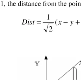
(5)Apparently, f(d)=0 is the separate line in a two-dimensional space with X and Y being X-coordinate and Y-coordinate. In this space, a given document d can be viewed as a point (x, y), in which the values of x and y are calculated according to (3) and (4).
As shown in Fig.1, the distance from the point (x, y) to the separate line will be:
)
(
2
1
Con
y
x
Dist
=
−
+
(6)Fig. 1. Distance from point (x, y) to the separate line
Fig. 2 illustrates the distribution of a training set (refer to Section 2.2) regarding Dist in the two-dimensional space, with the curve on the left for the negative samples, and the curve on the right for the positive samples. As can be seen in the figure, most of the misclassified documents, which unexpectedly across the separate line, are near the line. The error rate of the classifier is heavily influenced by this area, though the documents falling into this area only constitute a small portion of the training set.
Thus, the space can be partitioned into reliable area and unreliable area:
where Dist1 and Dist2 are constants determined by experiments, Dist1 is positive real
number and Dist2 is negative real number.
In the second step, more subtle and powerful features will be designed in particular to tackle the unreliable area identified in the first step.
2.2 Experiments on the Two-Class TC
The dataset used here is composed of 12,600 documents with 1,800 negative samples of TARGET and 10,800 positive samples of Non-TARGET. It is split into 4 parts randomly, with three parts as training set and one part as test set. All experiments in this section are performed in 4-fold cross validation.
CSeg&Tag3.0, a Chinese word segmentation and POS tagging system developed by Tsinghua University, is used to perform the morphological analysis for Chinese texts. In the first step, Chinese words with parts-of-speech verb, noun, adjective and adverb are considered as features. The original feature set is further reduced to a much smaller one according to formula (8) or (9). A Naïve Bayesian Classifier is then ap-plied to the test set. In the second step, only the documents that are identified unreli-able in terms of (7) in the first step are concerned. This time, bigrams of Chinese words with parts-of-speech verb and noun are used as features, and the Naïve Bayes-ian Classifier is re-trained and applied again.
∑
We try five methods as follows.
Method-1: Use Chinese words as features, reduce features with (9), and classify documents directly without exploring the two-step strategy.
Method-2: same as Method-1 except feature reduction with (8). Method-3: same as Method-1 except Chinese word bigrams as features.
Method-4: Use the mixture of Chinese words and Chinese word bigrams as fea-tures, reduce features with (8), and classify documents directly.
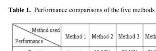
Note that the proportion of negative samples and positive samples is 1:6. Thus if all the documents in the test set is arbitrarily set to positive, the precision will reach 85.7%. For this reason, only the experimental results for negative samples are consid-ered in evaluation, as given in Table 1. For each method, the number of features is set by the highest point in the curve of the classifier performance with respect to the number of features (For the limitation of space, we omit all the curves here). The numbers of features set in five methods are 4000, 500, 15000, 800 and 500+3000 (the first step + the second step) respectively.
Table 1. Performance comparisons of the five methods in two-class TC
Comparing Method-1 and Method-2, we can see that feature reduction formula (8) is superior to (9). Moreover, the number of features determined in the former is less than that in the latter (500 vs. 4000). Comparing Method-2, Method-3 and Method-4, we can see that Chinese word bigrams as features have better discriminating capabil-ity meanwhile with more serious data sparseness: the performances of Method-3 and Method-4 are higher than that of Method-2, but the number of features used in Method-3 is more than those used in Method-2 and Method-4 (15000 vs. 500 and 800). Table 1 shows that the proposed method (Methond-5) has the best performance (95.54% F1) and good efficiency. It integrates the merit of words and word bigrams. Using words as features in the first step aims at its better statistical coverage, -- the 500 selected features in the first step can treat a majority of documents, constituting 63.13% of the test set. On the other hand, using word bigrams as features in the sec-ond step aims at its better discriminating capability, although the number of features becomes comparatively large (3000). Comparing Method-5 with Method-2, Method-3 and Method-4, we find that the two-step approach is superior to either using only one kind of features (word or word bigram) in the classifier, or using the mixture of two kinds of features in one step.
3 Extending the Two-Step Approach to the Multi-class TC
3.1 Fix the Fuzzy Area Between Categories by the Multi-class Bayesian Classifier
For a document represented by a binary-valued vector d = (W1, W2, …, W|D|), the
multi-class Naïve Bayesian Classifier can be re-written as:
∑
|C|), C is the number of predefined categories. Let:
∑
=
second_max
imum(
)
max_ (13)
where MVi stands for the likelihood of assigning a label ci∈C to the document d,
MVmax_F and MVmax_S are the maximum and the second maximum over all MVi
(i∈|C|) respectively. We approximately rewrite (10) as:
S F
MV
MV
d
f
(
)
=
max_−
max_ (14)We try to transfer the multi-class TC described by (10) into a two-class TC de-scribed by (14). Formula (14) means that the binary-valued multi-class Naïve Bayes-ian Classifier can be approximately regarded as searching a separate line in a two-dimensional space with MVmax_F being the X-coordinate and MVmax_S being the
Y-coordinate. The distance from a given document, represented as a point (x, y) with the values of x and y calculated according to (12) and (13) respectively, to the separate line in this two-dimensional space will be:
Dist = (x−y) 2 1
(15)
The value of Dist directly reflects the degree of confidence of assigning the label c* to the document d.
The distribution of a training set (refer to Section 3.2) regarding Dist in this two-dimensional space, and, consequently, the fuzzy area for the Naïve Bayesian Classi-fier, are observed and identified, similar to its counterpart in Section 2.2.
3.2 Experiments on the Multi-class TC
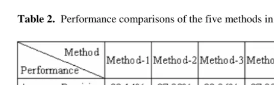
1800 respectively, among which the last three categories have the high degree of ambiguity each other. The dataset is split into four parts randomly, one as the test set and the other three as the training set. We again run the five methods described in Section 2.2 on this dataset. The strategy of determining the number of features also follows that used in Section 2.2. The experimentally determined numbers of features regarding the five methods are 8000, 400, 5000, 800 and 400 + 9000 (the first step + the second step) respectively.
The average precision, average recall and average F1 over the five categories are
used to evaluate the experimental results, as shown in Table 2.
Table 2. Performance comparisons of the five methods in multi-class TC
We can see from Table 2 that the very similar conclusions as that in the two-class TC in Section 2.2 can be obtained here:
1) Formula (8) is superior to (9) in feature reduction. This comes from the formance comparison between Method-2 and Method-1: the former has higher per-formance and higher efficiency that the latter (the average F1, 97.20% vs. 91.48%, and
the number of features used, 400 vs. 8000).
2) Word bigrams as features have better discriminating capability than words as features, along with more serious data sparseness. The performances of Method-3 and Method-4, which use Chinese word bigrams and the mixture of words and word bi-grams as features respectively, are higher than that of Method-2, which only uses Chinese words as features. But the number of features used in Method-3 is much more than those used in Method-2 and Method-4 (5000 vs. 400 and 800).
3) The proposed method (Methond-5) has the best performances and acceptable ef-ficiency. In term of the average F1, the performance is improved from the baseline
91.48% (Method-1) to 98.56% (Method-5). In the first step in Method-5, the number of feature set is small (only 400), but a majority of documents can be treated by it. The number of features exploited in Method-5 is the highest among the five methods (9000), but it is still acceptable.
4 Using Dependences Among Features in Two-Step
Categorization
second step, each document identified unreliable in the first step are further processed by exploring the dependences among features. This is realized by a model named the Causality Naïve Bayesian Classifier.
4.1 The Causality Naïve Bayesian Classifier (CNB)
The Causality Naïve Bayesian Classifier (CNB) is an improved Naïve Bayesian Clas-sifier. It contains two additional parts, i.e., the k-dependence feature list and the fea-ture causality diagram. The former is used to represent the dependence relation among features, and the latter is used to estimate the probability distribution of a feature dynamically while taking its dependences into account.
K-Dependence Feature List (K-DFL): CNB allows each feature node Y to have a maximum of k features nodes as parents that constitute the k-dependence feature list representing the dependences among features. In other words, ∏(Y) = {Yd, C}, where
Yd is the set of at most k features nodes, C is the category node, and ∏(C) =Φ.
Note that we can build a K-DFL for each feature under each class ct, which
repre-sents different dependence relations under different class.
Obviously, there exists a 0-dependence feature list for every feature in the Naïve Bayesian Classifier, from the definition of K-DFL.
The algorithm of constructing K-DFL is as follows: Given the maximum depend-ence number k, mutual information threshold θ and the class ct. For each feature Y,
repeat the follow steps. 1) Compute class conditional mutual information MI(Yi, Yj|
ct), for every pair of features Yi and Yj, where i≠j. 2) Construct the set Si={ Yj |
MI(Yi, Yj| ct) > θ}. 3) Let m= min (k, | Si|), select the top m features as K-DFL
from Si.
Feature Causality Diagram (FCD): CNB allows each feature Y, which occurs in a given document, to have a Feature Causality Diagram (FCD). FCD is a double-layer directed diagram, in which the first layer has only the feature node Y, and the second layer allows to have multiple nodes that include the class node C and the correspond-ing dependence node set S of Y. Here, S=Sd∩SF, Sd is the K-DFL node set of Y and
SF={Xi| Xi is a feature node that occurs in the given document. There exists a directed
arc from every node Xi at the second layer to the node Y at the first layer. The arc is
called causality link event Li which represents the causality intensity between node Y
and Xi, and the probability of Li is pi=Pr{Li}=Pr{Y=1|Xi=1}. The relation among all
arcs is logical OR. The Feature Causality Diagram can be considered as a sort of simplified causality diagram [9][10].
Suppose feature Y’s FCD is G, and it parent node set S={X1, X2,…,Xm } (m≥1) in
G, we can estimate the conditional probability as follows while considering the de-pendences among features:
∑
∏
= −
= =
− +
= =
= ≅ = =
= m
i i j
j i
i
i p p p
2 1
1 1
m
1 m
1 1, ,X 1} Pr{Y 1|G} Pr{ L} (1 )
X | 1
Pr{Y L
U
(16)Causality Naïve Bayesian Classifier (CNB): For a document represented by a bi-nary-valued vector d=(X1 ,X2 , …,X|d|), divide the features into two sets X1 and X2,
X1= {Xi| Xi=1} and X2= {Xj| Xj=0}. The Causality Naïve Bayesian Classifier can be
written as:
})) c | {X Pr log(1 }
G | logPr{X }
(logPr{c max
arg c*
| |
1 |
|
1
t j j
i
i i t
C ct
∑
∑
= =
∈ + + −
=
2 1
X X
(17)
4.2 Experiments on CNB
As mentioned earlier, the first step remains unchanged as that in Section 2 and Sec-tion 3. The difference is in the second step: for the documents identified unreliable in the first step, we apply the Causality Naïve Bayesian Classifier to handle them.
We use two datasets in the experiments. one is the two-class dataset described in Section 2.2, called Dataset-I, and the other one is the multi-class dataset described in Section 3.2, called Dataset-I.
To evaluate CNB and compare all methods presented in this paper, we experiment the following methods:
1) Naïve Bayesian Classifier (NB), i.e., the method-2 in Section 2.2; 2) CNB without exploring the two-step strategy;
3) The two-step strategy: NB and CNB in the first and second step (TS-CNB); 4) Limited Dependence Bayesian Classifier (DNB) [11];
5) Method-5 in Section 2.2 and Section 3.2 (denoted TS-DF here).
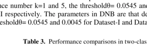
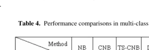
Experimental results for two-class Dataset-I and multi-class Dataset-II are listed in Table3 and Table 4. The data for NB and TS-DF are derived from the corresponding columns of Table 1 and Table 2. The parameters in CNB and TS-CNB are that the dependence number k=1 and 5, the thresholdθ= 0.0545 and 0.0045 for Dataset-I and Dataset-II respectively. The parameters in DNB are that dependence number k=1and 3, the thresholdθ= 0.0545 and 0.0045 for Dataset-I and Dataset-II respectively.
Table 3. Performance comparisons in two-class Dataset-I
identified reliable by NB, CNB cannot improve it, but for those identified unreliable by NB, CNB can improve it. The reason should be even though NB and CNB use the same features, but CNB uses the dependences among features additionally. 2) CNB and TS-CNB have the same capability in effectiveness, but TS-CNB has a higher computational efficiency. As stated earlier, TS-CNB uses NB to classify documents in the reliable area and then uses CNB to classify documents in the unreliable area. At the first glance, the efficiency of TS-CNB seems lower than that of using CNB only because the former additionally uses NB in the first step, but in fact, a majority of documents (e.g., 63.13% of the total documents in dataset-I) fall into the reliable area and are then treated by NB successfully (obviously, NB is higher than CNB in effi-ciency) in the first step, so they will never go to the second step, resulting in a higher computational efficiency of CNB than CNB. 3) The performances of CNB, TS-CNB and DNB are almost identical, among which, the efficiency of TS-TS-CNB is the highest. And, the efficiency of CNB is higher than that of DNB, because CNB uses a simpler network structure than DNB, with the same learning and inference formalism. 4) TS-DF has the highest performance among the all. Meanwhile, the ranking of computational efficiency (in descending order) is NB, TS-DF, TS-CNB, CNB, and DNB.
Table 4. Performance comparisons in multi-class Dataset-II
5 Related Works
6 Conclusions
The issue of how to classify Chinese documents characterized by high degree ambi-guity from text categorization’s point of view is a challenge. For this issue, this paper presents two solutions in a uniform two-step framework, which makes use of the distributional characteristics of misclassified documents, that is, most of the misclas-sified documents are near to the separate line between categories. The first solution is a two-step TC approach based on the Naïve Bayesian Classifier. The second solution is to further introduce the dependences among features into the model, resulting in a two-step approach based on the so-called Causality Naïve Bayesian Classifier. Ex-periments show that the second solution is superior to the Naïve Bayesian Classifier, and is equal to CNB without exploring two-step strategy in performance, but has a higher computational efficiency than the latter. The first solution has the best per-formance in all the experiments, outperforming all other methods (including the sec-ond solution): in the two-class experiments, its F1 increases from the baseline 82.67%
to the final 95.54%, and in the multi-class experiments, its average F1 increases from
the baseline 91.48% to the final 98.56%.
In addition, the other two conclusions can be drawn from the experiments: 1) Us-ing Chinese word bigrams as features has a better discriminatUs-ing capability than usUs-ing words as features, but more serious data sparseness will be faced; 2) formula (8) is superior to (9) in feature reduction in both the two-class and multi-class Chinese text categorization.
It is worth point out that we believe the proposed method is in principle language independent, though all the experiments are performed on Chinese datasets.
Acknowledgements
The research is supported in part by the National 863 Project of China under grant number 2001AA114210-03, 2003 Korea-China Young Scientists Exchange Program, the Tsinghua-ALVIS Project co-sponsored by the National Natural Science Founda-tion of China under grant number 60520130299 and EU FP6, and the NaFounda-tional Natu-ral Science Foundation of China under grant number 60321002.
References
1. Sebastiani, F. Machine Learning in Automated Text Categorization. ACM Computing Sur-veys, 34(1):1-47, 2002.
2. Lewis, D. Naive Bayes at Forty: The Independence Assumption in Information Retrieval. In Proceedings of ECML-98, 4-15, 1998.
3. Salton, G. Automatic Text Processing: The Transformation, Analysis, and Retrieval of In-formation by Computer. Addison-Wesley, Reading, MA, 1989.
4. Mitchell, T.M. Machine Learning. McCraw Hill, New York, NY, 1996.
5. Yang, Y., and Liu, X. A Re-examination of Text Categorization Methods. In Proceedings of SIGIR-99, 42-49,1999.
7. Dumais, S.T., Platt, J., Hecherman, D., and Sahami, M. Inductive Learning Algorithms and Representation for Text Categorization. In Proceedings of CIKM-98, Bethesda, MD, 148-155, 1998.
8. Sahami, M., Dumais, S., Hecherman, D., and Horvitz, E. A. Bayesian Approach to Filter-ing Junk E-Mail. In LearnFilter-ing for Text Categorization: Papers from the AAAI Workshop, 55-62, Madison Wisconsin. AAAI Technical Report WS-98-05, 1998.
9. Xinghua Fan. Causality Diagram Theory Research and Applying It to Fault Diagnosis of Complexity System, Ph.D. Dissertation of Chongqing University, P.R. China, April 2002. (In Chinese)
10. Xinghua Fan, Zhang Qin, Sun Maosong, and Huang Xiyue. Reasoning Algorithm in Multi-Valued Causality Diagram, Chinese Journal of Computers, 26(3), 310-322, 2003. (In Chinese)
11. Sahami, M. Learning Limited Dependence Bayesian Classifiers. In Proceedings of the Second International Conference on Knowledge Discovery and Data Mining, Portland, 335-338, 1996.
12. Rajashekar, T. B. and Croft, W. B. Combining Automatic and Manual Index Representa-tions in Probabilistic Retrieval. Journal of the American society for information science, 6(4): 272-283,1995.
13. Yang, Y., Ault, T. and Pierce, T. Combining Multiple Learning Strategies for Effective Cross Validation. In Proceedings of ICML 2000, 1167–1174, 2000.
14. Hull, D. A., Pedersen, J. O. and H. Schutze. Method Combination for Document Filtering. In Proceedings of SIGIR-96, 279–287, 1996.
15. Larkey, L. S. and Croft, W. B. Combining Classifiers in Text Categorization. In Proceed-ings of SIGIR-96, 289-297, 1996.
16. Li, Y. H., and Jain, A. K. Classification of Text Documents. The Computer Journal, 41(8): 537-546, 1998.
17. Lam, W., and Lai, K.Y. A Meta-learning Approach for Text Categorization. In Proceed-ings of SIGIR-2001, 303-309, 2001.