An integrated method for the quantity to be ordered to supplier

(1)

3rd National Conference on Recent Trends & Innovations In Mechanical Engineering 15th & 16th March 2019

Available online at www.ijrat.org

An Integrated Method for the Quantity to be ordered to

Supplier

1

Karuna Kumar .G 2 Dr. B.KarunaKumarb 3Dr. KesavaRaoV. V. S 1

Assistant professor, 2 Professor, 3 Professor

1

Assistant professor , Department of Mechanical Engineering , Gudlavalleru Engineering College, Gudlavalleru, Andhra Pradesh 521356, India

2

Professor, Department of Mechanical Engineering , Gudlavalleru Engineering College, Gudlavalleru, Andhra Pradesh 521356, India

3

Professor, Department of Mechanical Engineering , Andhra University College of Engineering, Visakhapatnam A.P., India.

Abstract: Supplier selection is an essential task within the purchasing function. A well-selected set of suppliers makes a strategic deference to an organization’s ability to reduce costs and improve the quality of its end products. This realization drives the search for new and better ways to evaluate and select suppliers. The correlated Analytic Hierarchy considers the correlation effect between criteria in the Analytic Hierarchy process. Linear physical programming(LPP) is a multi - objective opti mization method that develops an aggregate objective function of the criteria in a piecewise, goal - programming fashion. In order to think about multiple criteria LPP model allows decision maker (i.e., cost, customer service, and rejections) and to express criteria preferences in terms of degrees of desirability. This paper highlights an integrated method for dealing with such problems using correlat ed Analytic Hierarchy and linear physical programming techniques. The proposed method demonstrates selection of appropriate suppliers and allocates orders optimally among them

This paper proposes an integrated method for dealing with such problems using correlated Analytic Hierarchy– and linear physical programming techniques. The method proposed demonstrates selection of appropriate suppliers and allocates orders optimally among them finally model calculation is presented.

Index Terms - Correlated AHP ,linear physical programming, supplier selection, order allocation

1.

INTRODUCTION

Today, organizations that wish to sustain growing path requires a robust strategic performance measurement and evaluation system . one of the important function of the purchasing decision makers is Supplier selection with order allocation, which determines the long - term viability of the company a good supplier selection makes a significant difference to an organization’s future to reduce operational costs and improve the quality of its end products. in addition to this selling the product in a right market is equally important . hence in supply chain the transport of goods movement plays vital role. generally companies either on their own transport material with their fleet or through logistic suppliers. selection of right logistic supplier impacts the performance of the compa ny as it involves time, money, customer preference. Competitive advantage stems from the many discrete activities a company performs in designing, producing, marketing, delivering, and supporting its products.

The objective of the study includes Identifying the criteria for supplier selection Study of the factors whether they influence each other to find the correlation matrix between the criteria To find the weights considering the correlation by multi objective programming. To find the relative weight age factors to find the scores among the suppliers using AHP the quantity to be ordered on each supplier using linear physical programming.

2. LITERATURE SURVEY

There are comprehensive literature reviews performed for supplier selection application by Dickson [5], Weber et al.

[6], De Boer et al. [7] and Sanayei et al. [8]. Ayhan [9]. Dickson‟s [4] stated 23 creteria for supplier selection.

Cheraghi et al. [10] updated Dickson‟s criteria with 13 more . As a brief of all criteria price, quality, and delivery performances are found as the most significant selection criteria s. various multi criteria decision making methods are put into practice , which can be catagorised broadly into into three

1) Value Models: AHP and multi attribute utility theory (MAUT) fall in this group.

2) Goal, Models: Goal programming , TOPSIS.VIKOR belong to the group.

(2)

[16] cited a comprehensive study of the product recovery in manufacturing industry .. Kongar and Gupta [17] presented a multi-criteria decision making approach where the objective was to find the best combination of EOL products. Imtanavanich and Gupta [18] modeled the supply chain problem with stochastic yields using multi-criteria decision making approach LPP technique is used in solving the supply chain problem by Imtanavanich and Gupta [19]. Massoud and Gupta [20] considered the multi-period order problem .Kongar and Gupta [21] focused for EOL electronic products and proposed a LPP model taking into account environmental, performance and financial goals

3. METHODOLOGY

The study is done in three phases for supplier selection. Before proceeding to various phases the various factors for supplier selection is considered in the phase one the inter relation ship among factors is considered. In the second phase the weights among the factors considered. In the third phase linear physical programming is considered.

Mathematical model: In this paper, The supplier selection

is followed by a process depicted in as per the flow diagram mentioned below.

Analytic hierarchy process was proposed by Saaty based on multiple attributes in a hierarchical system. It should be highlighted that all decision problems are considered as a hierarchical structure in the AHP.

In the second level, the goal is decomposed of several criteria and the lower levels divide into other sub criteria. Therefore, the general form of AHP can be illustrated as shown in Fig ure2. A.H.P. Analytic hierarchy process was suggested by Saaty to model subjective decision making processes based on multiple attributes in a hierarchical system. It has been widely used in corporate planning, portfolio selection, and benefit/cost analysis by government agencies for resource allocation purposes from that time onwards. It should be focused that all decision problems are considered as a hierarchical structure in the AHP. The initial level indicates the goal for the specific decision problem. In the second level, the goal is decomposed of several criteria and the lower levels can follow this principal to divide into other sub criteria. Accordingly, the general form of AHP can be depicted as shown in in Figure2.

.

Fig. 2: The hierarchical structure of AHP

The main four steps of the AHP can be summarized as follows:

Step-1: Set up the hierarchical system by decomposing the

problem into a hierarchy of interrelated elements/criteria.

Step-2: Compare the comparative weight between the

attributes of the decision elements to form the reciprocal matrix.

Step-3: Synthesize the individual subjective judgment and estimate the relative weight.

Step-4: Aggregate the relative weights of the elements to determine the best alternatives/strategies.

If we wish to compare a set of n attributes pairwise according to their relative weights (importance), where the weights are

W = [wij]n×n ,

where Wij = wij–1, wij= wikwkj and wij= wi/wj

1 1 1

1

1 1

1

j n

i i i

w j j

j n

n n

n n n

j n

w w w

w w

w w w

W w n w nw

w w w

w w

w w w

 

 

 _{ } _ _ _

 _{ } _ _ _

_  

    

 _{ } _ _ _

   

 

 

(3)

Next, in order to estimate the weight ratio wij by aij,

where A = [aij]n×n, we can calculate the approximate weights

by finding the eigenvector w with respect to max which

satisfies

Aw = ʎmaxw

where ʎmax is the largest eigenvalue of the matrix A. in

addition , since A is an approximate for W, we should calculate the consistency indexes (C.I.) to check if the consistency condition is almost satisfied for A using the following equation:

C.I = max

1

n





where ʎmax is the largest eigenvalue and n denotes the

numbers of the attributes. Satty suggested that the value of the C.I. should not exceed 0.1 for a confident result.

On the other hand, for the AHP, a near consistent matrix A with a small reciprocal multiplicative perturbation of a consistent matrix is given by

A = WE,

where  denotes the Handmard product, W = [wij]n×n is the

matrix of weight ratios, and E = [ij]n×n is the perturbation

matrix, where ij =

1

ij





.

From (4) and (6) it can be seen that

max 1

0

n

ij j i

j

a w

w











(1)

max

1 1

n n

j

ij ij

j i j

w

a

w

 













(2)

On the other hand, the multiplicative perturbation can be transformed to an additive perturbation of a consistent matrix such that

1 1

n n

i i

ij ij

j j j j

w

v

w

 











(3)

where vij is the additive perturbation.

Since

1

n n

ij j i ij

j

a w w



j





, we can rewrite (8) as

1 1 1

1 1

,

.

n n n

j

i i i

ij ij ij

j j i j j j j

n n

i ij ij

j j j

w

w w w

a v

w w w w

w v a w                                    _  _  



 ₍₄₎

On the basis of (8)-(10), it can be seen that max = n if and

only if all ij =1 or vij=0, which is equivalent to having all aij

= wi/wj, indicates the consistent situation. Therefore, the

problem of deriving the relative weights among criteria in

the AHP is equivalent to solving the following mathematical programming to obtain wi:

Min

1

n

i ij

j j _p

w

a

w







s.t 1

1,

n i i

w





1  i

n (5)

where

.

_pdenotes the p-norm and p



{1,2,….}.

Correlated AHP

Although the AHP is widely used in the field of decision making, it cannot deal with the situation of correlation between criteria. Hence, we propose the extension of the AHP by considering the correlation between criteria.

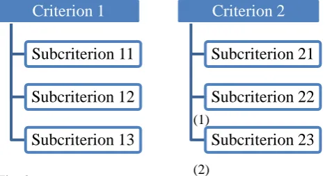
[image:3.595.318.552.313.440.2]

Fig. 3:

According to the presentation of Fig.3it can be identified that Criteria 1 and 2 are considered to change the decision of the problem. Criterion 1 can be divided into 3 independent sub criteria and so can Criterion 2. We should highlight that since Criteria 1 and 2 are correlated with each other, this problem cannot be solved neither by the AHP nor by the ANP. In order to consider the correlation effect in the AHP, we should first quantify the correlation matrix between criteria which is given by an expertise. Take Fig.3 as the example. We can rewrite the above correlation matrix or we can obtain the following correlation matrix. we should first quantify the correlation matrix between criteria which is given by an expertise. Take Fig.3 as the example.

We can obtain the following correlation matrix

11 12 13 14 15 16

21 22 23 24 25 26

31 32 33 34 35 36

41 42 43 44 45 46

51 52 53 54 55 56

61 62 63 64 65 66

r r r r r r

R

r r r r r r

(4)

or we can rewrite the above correlation matrix as,

where

11 12 13

11 21 22 23

31 32 33

r

R

r









 











,

14 15 16

12 24 25 26

34 35 36

r

R

r









 











,

44 45 46

11 54 55 56

64 65 66

r

R

r









 











Self-correlation effect:

Note that the self-correlation effect could happen in other situations. In addition, it should be highlighted that Rji

= Rij, i,j, because the correlation effect is symmetric.

Then, we assume that if Criterion i is highly correlated to Criterion j, they have similar weights or influence to the problem. Hence, if we obtain the correlation matrix between criteria, we can objective to maximize the correlation, that is, Rw.

4. LINEAR PHYSICAL PROGRAMMING

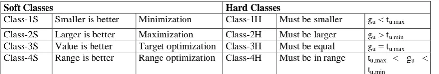
Linear Physical Programming (LPP), as a multi-objective optimization method, aggregates multi-objective function of the criteria in a piece-wise Archimedean goal programming style. Developed by Messac et al. [10], LPP simplifies physical programming procedure by defining preference functions as piece-wise linear functions [10]. LPP has been successfully applied to different multi-objective problems ma etc. [11]. LPP has the ability to avoid the weight assignment by providing a preference function. DM (decision maker) determines a suitable preference function and specifies ranges of different degrees of desirability (ideal, desirable, tolerable, undesirable, highly undesirable, and unacceptable) for each criterion the physical programming algorithm requires that the decision maker expresses his/her preferences with respect to each criterion using one of the eight different classes. The first four classes are “Soft class functions”, and represent minimization (Class-1S), maximization (Class-2S), value (Class 3S), and range (Class 4S) optimization. The remaining four are “Hard class functions” and are used to introduce inequality and range restrictions into the problem environment. In this regard, Class 1H and Class 2H define

[image:4.595.77.526.532.608.2]

upper and lower bounds, respectively, while Class 3H imposes equality and Class 4H imposes range related restrictions to the problem environment. The qualitative and quantitative depiction of each class is provided in Figures 1 and 2. The soft class functions allow the DM to express varying levels of preferences for each criterion. This is done by introducing corresponding constraints for each preference level in each of the classes. To provide better understanding, consider Class 1-S and Class 2-S, depicted in Figure 1, which are used for “Smaller is Better” and “Larger is Better” cases respectively. Table 1 demonstrates the ranges and corresponding constraints for the problem. Note that all the soft class functions will be embedded in the aggregate objective function to be minimized.

In Figure 1, the uth generic criterion is indicated as

gu(x) where x is the decision variable vector. The goal value,

gu is represented on the horizontal axis while, zu, the class

function that is subject to minimization is represented on the vertical axis. Since LPP algorithm considers the lower values of the class functions as “better” values but prohibits negative values, the class function that corresponds to the ideal value is set to zero.

Table 1

Soft Classes Hard Classes

Class-1S Smaller is better Minimization Class-1H Must be smaller gu < tu,max

Class-2S Larger is better Maximization Class-2H Must be larger gu > tu,min

Class-3S Value is better Target optimization Class-3H Must be equal gu = tu,max

Class-4S Range is better Range optimization Class-4H Must be in range tu,max < gu <

tu,min Model : To identify the key selection criteria in a

manufacturing industry in order to place orders on on each manufacturer called as supplier a considerable study was conducted. Constructed a decision hierarchy, identified the factors whether they influence each other to find the correlation matrix between the criteria. Normalized weights of factors are found considering the correlation by multi objective programming. the scores among the suppliers using correlated a hp are found. Finally the quantity to be ordered on each supplier using LPP taking into consideration of target level s ore obtained

Phase one :The selection of criteria scores are obtained as

per satty guide lines

.ahp weight calculation: The meaning of the terminology used.

 Operation speed: . It indicates generally which supplier will deliver fast because of the process capability

 Operating Readiness: Preparation of stores which can be used straightaway without a bit of damage.

 Operation accuracy: It includes many aspects like adherence to transportation time, on-time delivery

 Order processing: Order processing starts from picking, packaging and packed items delivery

 Operating cost: Operating costs are the expenses for conducting the a business or facility

41 42 43

21 51 52 53

61 62 63

r

R

r









 







(5)

 Storage cost &Transportation cost: it includes the cost of moving and storing possessions

 Information technology: it is the application of computers and data acquisition and data management for conduct of business or other manufacturing and allied activities.

 Storage Technology: the technology implemented for storage

 Transportation technology: the technology implemented for transporting

 Customer satisfaction: It is a measure of how goods and services supplied by a company

 Compatibility : it is the ability of the manufacturer, its vendors and their customers work in collaboration

 Financial easiness: Ensures continuity in services., better cash flow, sound balance sheet are indicators Table2 : Factors of suppliers selection

Operating efficiency (B1):

C1. Operation speed C2. Operating readiness C3. Operation accuracy

Cost(B2)

C4. Transportation cost C5. Storage cost

C6. Order processing cost

Technology level satisfaction (B3):

C7. Information technology C8. Storage technology C9.Transportation technology

Service Quality (B4)

C10. Customer satisfaction C11. Compatibility C12.Financial easiness .

operating efficiency, cost, technology level and service quality are represented by B1, B2, B3 and B4 respectively.

Step 1:column sum s( table 5). After considering the relations between different aspects .the column Sum for the normalization

purpose is performed.,ex Sum 1 = B11+B21+B31+B41 = 1+0.5+0.333+0.5 = 2.3333

Step2: column normalization see table 6: B11= ⁄=0.4285; … the remaining all calculated.

Step3: Row sums (table 7):row wise totalling ex Sum1 =

(0.4285+0.4444+0.375+0.4444) = 1.6923 .

Step4: (table 8). The individual row sums are divided by the

total sum to get weights.W1 = s1/s = 1.69/3.99 = 0.4231

Step5:Consistencyindex:The consistency index (CI)

measures the consistency set of data. consistence ratio (cr).oo4 which is acceptable for first level. Ahp weights are considered for next level B1,B2,B3,B4Phase 2:7.2 : Correlation Matrix :By considering individual operation speed and corresponding Order processing cost rate are in correlation with each other (table 14).The correlation is

calculated as mentioned below. The correlation coefficient is r =

√( )( ) =

√( )( ) =0.213 ≈ 0.2all correlation

coefficients(table13)

(6)

Table8: Row normalization of the factors Table 9: Relation between internal factors of B1

A B1 B2 B3 B4 Weights

B1 0.4285 0.4444 0.375 0.4444 0.4231 B2 0.2142 0.2222 0.25 0.2222 0.2271 B3 0.1428 0.1111 0.125 0.1111 0.1225 B4 0.2142 0.2222 0.25 0.2222 0.2271

B1 C1 C2 C3 Normal ahp Weights

C1 1 3 2 0.55

C2 1/3 1 1 0.21

C3 ½ 1 1 0.2422

. Table 9the consistency ratio are found in order Cr = .001

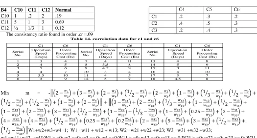
[image:6.595.35.561.351.634.2]

The table 10 consistency ratio are found in order Cr =.001Table 11 the consistency ratio found in order . Cr =.05

Table 12: Relation between internal factors of B4 Table 13 correlation table

B4 C10 C11 C12 Normal

ahpweightsahpW

C10 1 .2 2 .19 C11 5 1 3 0.69 C12 ½ 1/3 1 0.12

The consistency ratio found in order .cr =.09

Table 14. correlation data for c1 and c6

C1 C6 C1 C6 C1 C6

Serial No.

Operation Speed (Days)

Order Processing

Cost (Rs)

Serial No.

Order Processing

Cost (Rs)

Serial No.

Order Processing

Cost (Rs)

1 3 4 7 4 11 13 4 8

2 4 5 8 3.5 8 14 5 9

3 5 6 9 4.5 9 15 3 11

4 4 7 10 3 4 16 4 10

5 5.5 10 11 4 5 17 3 7

6 3 9 12 5 7 18 4.5 8

Min m = -‖( ) ( ) ( _{) (}⁄ ) ( ) ( _{) (}⁄ _{) (}⁄ )

( ⁄ _{) (}⁄ ) ( ) ( )‖ ‖(

) (

) ( ⁄

) (

) ( ⁄ )

(

) (

) ( ⁄

) (

) ( ⁄

) (

) ( )

(

) (

) ( ⁄

) (

) ( ⁄ )

( ⁄

)‖W1+w2+w3+w4=1; W1 =w11 + w12 + w13; W2 =w21 +w22 +w23; W3 =w31 +w32 +w33;

[image:6.595.43.491.680.737.2]

w4 =w41+w42 +w43;W1 > =0; w2 >=0; w3 >= 0; w4 >=0;W11 > =0; w12 >=0; w13 >= 0;W21 > =0; w22 >=0; w23 >= 0; W31 > =0; w32 >=0; w33 >= 0;W41 > =0; w42 >=0; w43 >= 0; Where w1 ,w2,w3,w4 are weights of b1,b2.b3,b4 respectively . and w11,w12,w13 w21,w22,w23,w31,w32,w33,w41,w42,w43are weights of c1,c2,c3,c4,c5,c6,c7,c8,c9,c10,c11,c12,c23 respectively.

Table 15.The results of correlated weights

Top-Level

Factors Weights

Second

Level Weights

Second

Level Weights

Second

Level Weights

B1 0.1142675 c1 0.062939 c5 0.04732 c9 0.029755

B2 0.1421024 c2 0.023208 c6 0.071051 c10 0.18665

B3 0.1814302 c3 0.027676 c7 0.060235 c11 0.2811

B4 0.5621999 c4 0.023731 c8 0.090715 c12 0.092201

The table(15) clearly demonstrates the correlated ahp values are different from normal ahp values. First normal ahp is perfor med to check the consistency.

C4 C5 C6

C1 .2 .3 .2

C2 .4 .5 .3

(7)

7.4 supplier wise ranks are calculated .Each supplier is given weight with respect to each factor. On a scale of 1 ---10.Supplier weights are calculatedin table 16 and 17

Table 16 Supplier global weighed scores

Phase 3

7.5 linear physical programming: the data considered for this part of section is mentioned in tables18,19,20.

7.6 Formulation of equation

Operating efficiency Goal = g1 = 0 .78 x1 +0.81 x2 +0.80 x3 + 0.81 x4

Technology satisfaction Goal = g2= 0.84 x1 +0.82 x2 +0.82 x3 +0.85 x4

service quality Goal = g3 = 0.7 x1 +0.7 x2 +0.5 x3 +0.6x4

cost Goal = g4 = 110 x1 +150 x2 +145 x3 +120 x4

Subject to Total quantity to be procuredx1 + x2 + x3 + x4= 1500 ;

the maximum limit that can be procured from supplier

x1<800 , x2<500 , x3<700 , x4<600 ; x1 ≥0 , x2 ≥0; , x3 ≥0 , x4 ≥0

x1 , x2, x3, x4 are the quantities to be ordered on suppliers1,2,3 and 4

5.5.2Based on linear physical programming, the equations are reformulated Objective function Min z = ∑ ̌ +̌ * +̌ *

Where ̌ ,̌ ̌ = weights calculated as per weighted algorithm

Table 17 .Supplier weighed scores of individual factors

Table 18 .Data of product

(8)

[image:8.595.159.436.124.193.2]

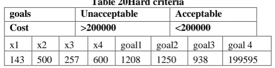
Table 20Hard criteria

goals Unacceptable Acceptable

Cost >200000 <200000

x1 x2 x3 x4 goal1 goal2 goal3 goal 4 143 500 257 600 1208 1250 938 199595

8. CONCLUSION

The problem is solved using software lingo 11 Multi objective technique is used to find out the correlated weights of criteria in supplier selection. Implementation of linear physical programming technique which has the capability to represent decision maker preference by using a utility function and to manage problem in multi criteria environment for order allocation is presented. The study gives ample scope for Future scope: such as The model can be further extended accommodating more variables such as power requirements infrastructure requirements, product recycling etc. this can be extended to new areas with fuzziness in consideration

Acknowledgment

I wish to thank Dr.B. Karuna Kumar and Dr. Kesava Rao V. V. S, who guided me with his suggestions on this paper and all the people at vizag steel plant who helped us with valuable information pertaining to Suppler selection for purchase department..

REFERENCES

[1] Chen, C. T., Lin, C. T., & Huang, S. F. (2006). A fuzzy approach for supplier evaluation & selection in supply chain management. International Journal of Production Economics, 102, 289–301.

[2] Ghodsypour, S. H., &O’brien, C. (2001). The total cost of logistics in supplier selection, under conditions of multiple sourcing, criteria and capacity constraint. International Journal of Production Economics, 73(1), 15–27.

[3] Hwang, C.L., and Yoon, K., (1981) Multiple Attribute Decision Making Methods and Applications: A State of the Art Survey, Springer-Verlag, USA

[4] Saaty, T.L., (1980)The Analytic Hierarchy Process, McGraw-Hill, New York, USA.

[5] Dickson,G.W.(1966)“An

AnalysisofVendorSelection Systems and Decision”.Journal ofPurchasingVol.2(1), 5-17. [6] Weber, C.A., Current J.R. and Benton, W.C.

(1991) “Vendor Selection Criteria and Methods”,European Journal of Operational Research Vol.50(1), 2-18.

[7] De Boer, L., Labro, E. and Morlacchi, P.,(2001) “A Review of Methods Supporting SuppliersSelection”,European Journal of

Purchasing and Supply Management Vol. 7(2), 75-89

[8] Sanayei, A., Mousavi, S.F. and Yazdankhak, A., (2010) “Group Decision Making Process forSuppliers Selection with VIKOR Under Fuzzy Environment”, Expert Systems with ApplicationsVol. 37 (1), 24-30.

[9] Ayhan, M.B. (2013). Fuzzy Topsis application for supplier selection problem. International

[10] Journal of Information, Business and Management, Vol. 5(2), 159-174.

[11] Cheraghi, S. H., Dadashzadeh,M., & Subramanian, M., (2004) “Critical success factors forSupplier selection: An Update”, Journal of Applied Business Research, Vol 20(2), 91–108.

[12] Ghodsypour, S.H., and O‟Brien, C., (1998) “A Decision Support System for Supplier Selection Using an Integrated Analytic Hierarchy Process and Linear Programming”, International Journal of Production Economics, Vol. 56-57(20), 199-212.. [13] Kilic, H.S., (2013) “An integrated approach for

supplier selection in multi item/multi supplier [14] environment”, Applied Mathematical Modelling,

Vol. 37 (14-15), 7752-7763.

[15] Xia, W. and Wu, Z., (2007) “Supplier selection with multiple criteria in volume discountenvironments”, Omega, Vol. 35(5), 494-504..

[16] Yahya, S. and Kingsman, B., (1999) “Vendor Rating for an Entrepreneur DevelopmentProgramme: A Case Study Using the Analytic Hierarchy Process Method”, Journal of theOperational Research Society Vol.50: 916-930. [17] Lambert, A. J. D. and Gupta, S. M., "Disassembly

Modeling for Assembly, Maintenance, Reuse, and Recycling," CRC Press, Boca Raton, Florida, ISBN: 1-57444-334-8, 2005.

[18] Gungor, A. and Gupta, S. M., "Issues in environmentally conscious manufacturing and product recovery: a survey," Computers & Industrial Engineering, Vol. 36, No. 4, 811-853, 1999.

[19] Kongar, E. and Gupta, S. M., "A multi-criteria decision making approach for disassembly-to-order systems," Journal of Electronics Manufacturing, Vol. 11, No. 2, 171-183, 2002.

(9)

system," Proceedings of the 2005 Northeast Decision Sciences Institute Conference, Philadelphia, Pennsylvania, 2005.

[21] Imtanavanich, P. and Gupta, S. M., "Evolutionary computation with linear physical programming for solving a disassembly-to-order system,"

Proceedings of the SPIE International Conference on Environmentally Conscious Manufacturing VI, Boston, Massachusetts, 30-41, 2006.

[22] Massoud, A. Z. and Gupta, S. M., "Solving the multi-period disassembly-to-order system under stochastic yields, limited supply, and quantity discount," Proceedings of 2008 ASME International Mechanical Engineering Congress and Exposition, Boston, MA, 2008.

[23] Kongar, E. and Gupta, S. M., "Solving the disassembly-to-order problem using linear physical programming," International Journal of Mathematics in Operational Research, Vol. 1, No. 4, 504-531, 2009.

[24] Hsiang-Hsi Liu, Yeong-YuhYeh, and Jih-JengHuang(2014) “Correlated Analytic Hierarchy Process” Mathematical Problems in EngineeringVolume 2014, Article ID 961714 [25] Fusunkucukbay and CeyhunAraz(2016) “ port folio

selection problem –a comparison of fuzzy goal programming and linear physical programming. an international journal of optimization and control theories and application vol 6 no 2 pp121-128 [26] Messac, A.; Gupta, S.; Akbulut, B. Linear Physical

Programming: A New Approach to Multiple Objective Optimization. // Transactions on Operational Research. 8, (1996), pp. 3959.

[27] Ma, X.; Dong, B. Linear Physical Programming-Based Approach for Web Service Selection. // Proceedings of the International Conference on Information Management, Innovation Management and Industrial Engineering, Taipei, Taiwan, (2008), pp. 398-401.

expenses

computers