Evaluating the Performance of Network Intrusion Detection System using Machine Learning Approaches

386

Evaluating the Performance of Network Intrusion

Detection System using Machine Learning Approaches

1

M. Srikanth Yadav,

M.C.P Saheb

Department of CSE

Tirumala Engineering College Narasaraopeta, Guntur, Andhra Pradesh, India

Abstract:Intrusion identification is a key piece of security devices, for example, versatile security apparatuses, interruption recognition frameworks, interruption counteractive action frameworks and firewalls. Different interruption location strategies are utilized; however their execution is an issue. Interruption identification execution relies upon precision, which needs to improve to diminish false alerts and to build the discovery rate. To determine worries on execution, Support vector machine (SVM), Naïve Bayes (NB) and Simple K-Nearest Neighbor (SKNN) methods have been utilized in late work. Such procedures show impediments and are not effective for use in huge datasets, for example, framework and system information. The interruption identification framework is utilized in investigating gigantic traffic information; therefore, a proficient characterization system is important to defeat the issue. This issue is considered in this paper. Understood machine learning procedures, specifically, SVM, Naïve Bayes, and Simple K-Nearest Neighbor are connected. These systems are notable as a result of their capacity in characterization. The NSL– learning disclosure and information mining dataset is utilized, which is viewed as a benchmark in the assessment of interruption discovery instruments.

Key Words: Naïve Bayes, NSL–KDD, Misuse, Simple K-Nearest Neighbors, Support vector machine

1. INTRODUCTION

Intrusion is a severe issue in security and a prime problem of security breach, because a single instance of intrusion can steal or delete data from computer and network systems in a few seconds. Intrusion can also damage system hardware. Furthermore, intrusion can cause huge losses financially and compromise the IT critical infrastructure, thereby leading to information inferiority in cyber war. Therefore, intrusion detection is important and its prevention is necessary.

Diverse interruption discovery methods are accessible, yet their precision remains an issue; exactness relies upon identification and false caution rate. The issue on exactness should be routed to decrease the bogus alerts rate and to expand the identification rate. This idea was the catalyst for this examination work. Therefore, support vector machine (SVM), Naïve Bayes (NB), and Simple k-Nearest Neighbors (SKNN) are connected in this work; these techniques have been demonstrated viable in their ability to address the order issue. Interruption recognition instruments are approved on a standard dataset, KDD. This work utilized the NSL– learning revelation and information mining (KDD) dataset, which is an improved type of the KDD and is viewed as a benchmark in the assessment of interruption recognition strategies.

The rest of the paper is sorted out as itemized underneath. The related work is introduced in Section II. The proposed model of

interruption location to which distinctive machine learning systems are connected is depicted in Section III. The usage and results are examined in Section IV. The paper is finished up in Section V, which gives an outline and headings to future work.

2. RELATED WORK

Verifying PC and system data is essential for associations and people on the grounds that bargained data can cause significant harm. To maintain a strategic distance from such conditions, interruption location frameworks are vital. As of late, extraordinary machine learning approaches have been proposed to improve the execution of interruption recognition frameworks. Wang et al. [1] proposed an interruption discovery system dependent on SVM and approved their strategy on the NSL– KDD dataset. They guaranteed that their strategy, which has 99.92% adequacy rate, was better than different methodologies; be that as it may, they didn't make reference to utilized dataset insights, number of preparing, and testing tests. Besides, the SVM execution diminishes when vast information are included, and it's anything but a perfect decision for examining enormous system traffic for interruption identification.

387 be one-sided to all the more every now and again

happening records. They connected KPCA for highlight decrease, and it is restricted by the likelihood of missing imperative highlights due to choosing top rates of the important part from the central space. Moreover, the SVM isn't suitable for overwhelming information, for example, observing the high data transmission of the system.

Interruption recognition frameworks give help with identifying, averting, and opposing unapproved get to. Therefore, Aburomman and Reaz [3] proposed a group classifier technique, which is a blend of PSO and SVM; this classifier beat different methodologies with 92.90% precision. They utilized the learning revelation and information mining 1999 (KDD99) dataset, which has the recently referenced downsides. Besides, the SVM is certainly not a decent decision for gigantic information examinations, since its execution debases as information estimate increments. Raman et al. [4] proposed an interruption discovery instrument dependent on hypergraph hereditary calculation (HG-GA) for parameter setting and highlight determination in SVM. They asserted that their technique outflanked the current methodologies with a 97.14 % discovery rate on a NSL– KDD dataset; it has been utilized for experimentation and approval of interruption recognition frameworks.

The security of system frameworks is a standout amongst the most basic issues in our day by day lives, and interruption recognition frameworks are huge as prime barrier methods. In this way, Teng et al. directed imperative work [5]. They built up their model dependent on choice trees (DTs) and SVMs,

and they tried their model on a KDD CUP 1999 dataset. The outcomes demonstrated a precision achieving 89.02%. Be that as it may, SVMs are not favored for substantial datasets on account of the high calculation cost and poor execution.

Farnaaz and Jabbar built up a model for an interruption recognition framework dependent on RF. They tried the viability of their model on a NSL– KDD dataset, and their outcomes exhibited a 99.67% discovery rate contrasted and J48 [6]. The principle confinement of the RF calculation is that numerous trees may make the calculation moderate for constant forecast.

Reda et al. [7] proposed a model of interruption identification dependent on RF and weighted k-implies; they approved their model over the KDD99 dataset. The framework exhibited outcomes with 98.3% exactness. The RF isn't reasonable for foreseeing genuine traffic on account of its gradualness, which is because of the arrangement of countless. Also, the KDD99 dataset demonstrates couple of confinements as previously mentioned.

3. PROPOSED MODEL

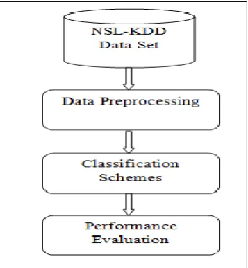
The key phases of the proposed model include the dataset, pre-processing, classification, and result evaluation. Each phase of the proposed system is important and adds valuable influence on its performance. The core focus of this work is to investigate the performance of different classifiers, namely, SVM, NB, and SKNN in intrusion detection. Figure 1 demonstrates the model of intrusion detection system proposed in this work.

Figure 1: Proposed Scheme of Evaluation

A. Dataset

Dataset determination for experimentation is a huge assignment, on the grounds that the execution of the framework depends on the accuracy of a dataset. The more precise the

388 happen in the use of the initial three systems. A

genuine traffic strategy is costly, while the purified technique is risky. The advancement of a reenactment framework is likewise unpredictable and testing. Furthermore, extraordinary sorts of traffic are required to display different system assaults, which is perplexing and exorbitant. To highlights. Consequently, pre-handling is basic, in which non-numeric or representative highlights are disposed of or supplanted, in light of the fact that they don't demonstrate crucial interest in interruption discovery. Be that as it may, this procedure creates overhead including all the more preparing time; the classifier's design winds up complex and squanders memory and processing assets. Thusly, the non-numeric highlights are prohibited from the crude dataset for enhanced execution of interruption location frameworks.

C. Classification

Setting an action into ordinary and nosy classes is the center capacity of an interruption recognition framework, which is known as a meddling investigation motor. Accordingly, extraordinary classifiers have been connected as meddling examination motors in interruption recognition in the writing, for example, multilayer perceptron, SVM, Naïve Bayes, self-sorting out guide, and DT. In any case, in this investigation, the three unique classifiers of SVM, NB, and SKNN are connected dependent on their demonstrated capacity in arrangement issues. Subtleties of every arrangement approach are given.

1. Support Vector Machines

Support Vector Machines are maybe a standout amongst the most prominent and discussed machine learning calculations. They were very prevalent around the time they were created during the 1990s and keep on being the go-to strategy for a high-performing calculation with small tuning. In this Paper you will find the Support Vector Machine (SVM) machine learning calculation. SVM is an energizing calculation and the ideas are moderately basic. This post was composed for engineers with practically zero foundation in measurements and straight variable based math.

a. Usage of M-M (Maximal-Margin) Classifier

The Maximal-Margin Classifier is a theoretical classifier that best clarifies how SVM functions practically speaking. The numeric information factors (x) in your information (the sections) structure a n-dimensional space. For

instance, on the off chance that you had two information factors, this would frame a two-dimensional space. A hyperplane is a line that parts the information variable space. In SVM, a hyperplane is chosen to best separate the focuses in the info variable space by their class, either class 0 or class 1. In two-measurements you can envision this as a line and how about we accept that the majority of our information focuses can be totally isolated by this line.

For instance: P0 + (P1 * Y1) + (P2 * Y2) = 0

Where the coefficients (P1 and P2) that decide the incline of the line and the block (P0) are found by the learning calculation, and Y1 and Y2 are the two information factors. We can make groupings utilizing this line. By connecting input qualities into the line condition, you can figure whether another point is above or underneath the line. Over the line, the condition restores an esteem more noteworthy than 0 and the point has a place with the top of the line. Underneath the line, the condition restores an esteem under 0 and the point has a place with the inferior. An esteem near the line restores an esteem near zero and the point might be hard to characterize.

b. Usage of S-M (Soft Margin) Classifier

In practice, real data is messy and cannot be separated perfectly with a hyperplane. The limitation of amplifying the edge of the line that isolates the classes must be loose. This is regularly called the delicate edge classifier. This change permits a few points in the preparation information to disregard the isolating line. An extra arrangement of coefficients are presented that give the edge squirm room in each measurement. These coefficients are some of the time called slack factors. This expands the intricacy of the model as there are more parameters for the model to fit to the information to give this unpredictability.

389 less delicate the calculation is to the preparation

information (lower fluctuation and higher predisposition).

c. Role of Kernels in SVM

The SVM calculation is actualized practically speaking utilizing a part. The learning of the hyperplane in straight SVM is finished by changing the issue utilizing some direct polynomial math, which is out of the extent of this prologue to SVM. A ground-breaking understanding is that the straight SVM can be reworded utilizing the internal result of any two given perceptions, instead of the perceptions themselves. The inward item between

two vectors is the entirety of the augmentation of each pair of information esteems. The condition for making an expectation for another information utilizing the dab item between the information (x) and each help vector (xi) is determined as pursues: f(y) = P0 + sum(bi * (y,yi))

This is a condition that includes figuring the inward results of another info vector (y) with all help vectors in preparing information. The coefficients P0 and bi (for each information) must be evaluated from the preparation information by the learning calculation.

Kernel Type Description

Linear Kernel SVM

The Kernel characterizes the likeness or a separation measure between new information and the help vectors. The speck item is the likeness measure utilized for direct SVM or a straight Kernel in light of the fact that the separation is a direct mix of the data sources. The spot item is known as the bit and can be re-composed as: K(y, yi) = sum(y * yi)

Polynomial Kernel SVM

Rather than the dot-product, we can utilize a polynomial kernel, for instance: K(y,yi) = 1 + sum(y * yi)^d. Where the level of the polynomial must be indicated by hand to the learning calculation. At the point when d=1 this is equivalent to the linear ker. The polynomial kernel takes into consideration curved lines in the info space.

Radial Kernel SVM

At long last, we can likewise have a progressively perplexing kernel. For instance: K(y,yi) = exp(- gamma * sum((y – yi^2)). Where gamma is a parameter that must be indicated to the learning calculation. A decent default value for gamma is 0.1, where gamma is regularly 0 < gamma < 1. The radial kernel is nearby and can make complex districts inside the component space, as shut polygons in two-dimensional space.

d How to Train SVM Model

The SVM model should be fathomed utilizing an advancement system. You can utilize a numerical streamlining strategy to look for the coefficients of the hyperplane. This is wasteful and isn't the methodology utilized in generally utilized SVM usage like LIBSVM. On the off chance that actualizing the calculation as an activity, you could utilize stochastic inclination plunge. There are particular improvement strategies that re-detail the streamlining issue to be a Quadratic Programming issue. The most prominent technique for fitting SVM is the Sequential Minimal Optimization (SMO) strategy that is extremely productive. It separates the issue into sub-issues that can be understood diagnostically instead of numerically.

e. Limitation of Data Preparation for SVM

This section records a few proposals for how to best set up your preparation information when learning a SVM model.

Numerical Inputs: SVM accept that your data sources are numeric. On the off chance that you have categorical input sources you may need to covert them to binary dummy variables.

Binary Classification: Basic SVM as depicted in this paper is proposed for binary (two-class) classification issues. Despite the fact that,

expansions have been created for regression and multi-class classification.

2. Naïve Bayes

Naive Bayes is a simple but surprisingly powerful algorithm for predictive modeling. In machine learning we are often interested in selecting the best hypothesis (h) given data (d). In a classification problem, our hypothesis (h) may be the class to assign for a new data instance (d). One of the easiest ways of selecting the most probable hypothesis given the data that we have that we can use as our prior knowledge about the problem. Bayes‟ Theorem provides a way that we can calculate the probability of a hypothesis given our prior knowledge. Bayes‟ Theorem is stated as:

P(h|d) = (P(d|h) * P(h)) / P(d)

Where P(h|d) is the probability of hypothesis h given the data d. This is called the posterior probability. P(d|h) is the probability of data d given that the hypothesis h was true. P(h) is the probability of hypothesis h being true (regardless of the data). This is called the prior probability of h. P(d) is the probability of the data (regardless of the hypothesis).

390 Naive Bayes is a classification algorithm

for binary (two-class) and multi-class classification problems. The technique is easiest to understand when described using binary or categorical input values. It is called naive Bayes or idiot Bayes because the calculation of the probabilities for each hypothesis is simplified to make their calculation tractable. Rather than attempting to calculate the values of each attribute value P(d1, d2, d3|h), they are assumed to be conditionally independent given the target value and calculated as P(d1|h) * P(d2|H) and so on. This is a very strong assumption that is most unlikely in real data, i.e. that the attributes do not interact. Nevertheless, the approach performs surprisingly well on data where this assumption does not hold.

b. Illustrations Used By Naive Bayes Models

The representation for naive Bayes is probabilities. A list of probabilities are stored to file for a learned naive Bayes model. This includes:

Class Probabilities: The probabilities of each class in the training dataset. Conditional Probabilities: The conditional probabilities of each input value given each class value. Learning a naive Bayes model from your training data is fast. Training is fast because only the probability of each class and the probability of each class given different input (x) values need to be calculated. No coefficients need to be fitted by optimization procedures.

c. Calculating Class Probabilities

The class probabilities are simply the frequency of instances that belong to each class divided by the total number of instances. For example in a binary classification the probability of an instance belonging to class 1 would be calculated as: P(class=1) = count(class=1) / (count(class=0) + count(class=1)). In the simplest case each class would have the probability of 0.5 or 50% for a binary classification problem with the same number of instances in each class.

d. Limitation in Preparation of Data for Naive Bayes

Type of Input Description

Categorical Inputs Naive Bayes assumes label attributes such as binary, categorical or nominal.

Gaussian Inputs

If the input variables are real-valued, a Gaussian distribution is assumed. In which case the algorithm will perform better if the univariate distributions of your data are Gaussian or near-Gaussian. This may require removing outliers (e.g. values that are more than 3 or 4 standard deviations from the mean).

Classification Problems Naive Bayes is a classification algorithm suitable for binary and multiclass classification.

Log Probabilities

The calculation of the likelihood of different class values involves multiplying a lot of small numbers together. This can lead to an underflow of numerical precision. As such it is good practice to use a log transform of the probabilities to avoid this underflow.

Kernel Functions Rather than assuming a Gaussian distribution for numerical input values, more complex distributions can be used such as a variety of kernel density functions.

Update Probabilities When new data becomes available, you can simply update the probabilities of your model. This can be helpful if the data changes frequently.

3. Simple K-Nearest Neighbor Model Representation

The model representation for KNN is the entire training dataset. It is as simple as that. KNN has no model other than storing the entire dataset, so there is no learning required. Efficient implementations can store the data using complex data structures like k-d trees to make look-up and matching of new patterns during prediction efficient. Because the entire training dataset is stored, you may want to think carefully about the consistency of your training data. It might be a good idea to curate it, update it often as new data becomes available and remove erroneous and outlier data.

a. Making Predictions with KNN

KNN makes predictions using the training dataset directly. Predictions are made for a new instance (y) by searching through the entire training

set for the K most similar instances (the neighbors) and summarizing the output variable for those K instances. For regression this might be the mean output variable, in classification this might be the mode (or most common) class value. To determine which of the K instances in the training dataset are most similar to a new input a distance measure is used. For real-valued input variables, the most popular distance measure is Euclidean distance. Euclidean distance is calculated as the square root of the sum of the squared differences between a new point (y) and an existing point (yi) across all input attributes j.

EuclideanDistance(y, yi) = sqrt( sum( (yj – yij)^2 ) )

391 input variables are not similar in type. The value

for K can be found by algorithm tuning. It is a good idea to try many different values for K and see what works best for your problem. The computational complexity of KNN increases with the size of the training dataset. For very large

training sets, KNN can be made stochastic by taking a sample from the training dataset from which to calculate the K-most similar instances. KNN has been around for a long time and has been very well studied. As such, different disciplines have different names for it, for example:

Types of KNN Learning Models Description

Instance-Based Learning

The raw training instances are used to make predictions. As such KNN is often referred to as instance-based learning or a case-based learning (where each training instance is a case from the problem domain).

Lazy Learning

No learning of the model is required and all of the work happens at the time a prediction is requested. As such, KNN is often referred to as a lazy learning algorithm

Non-Parametric

KNN makes no assumptions about the functional form of the problem being solved. As such KNN is referred to as a non-parametric machine learning algorithm.

b. KNN for Classification

When KNN is used for classification, the output can be calculated as the class with the highest frequency from the K-most similar instances. Each instance in essence votes for their class and the class with the most votes is taken as the prediction. Class probabilities can be calculated as the normalized frequency of samples that belong to each class in the set of K most similar instances for a new data instance. For example, in a binary classification problem.

p(class=0) = count(class=0) / (count(class=0)+count(class=1))

If you are using K and you have an even number of classes (e.g. 2) it is a good idea to choose a K value with an odd number to avoid a tie. And the inverse, use an even number for K when you have an odd number of classes. Ties can be broken consistently by expanding K by 1 and looking at the class of the next most similar instance in the training dataset.

c. Curse of Dimensionality

KNN works well with a small number of input variables (p), but struggles when the number

of inputs is very large. Each input variable can be considered a dimension of a p-dimensional input space. For example, if you had two input variables x1 and x2, the input space would be 2-dimensional. As the number of dimensions increases the volume of the input space increases at an exponential rate. In high dimensions, points that may be similar may have very large distances. All points will be far away from each other and our intuition for distances in simple 2 and 3-dimensional spaces breaks down. This might feel unintuitive at first, but this general problem is called the “Curse of Dimensionality“.

4. RESULTS

392 Table 1: Comparison of Classification Results

Measuring Parameter Classifier

SVM NB SKNN

Correctly Classified Instances 5656 (95.70%) 5625 (95.17 %) 5657 (95.71 %) Incorrectly Classified

Instances 254 (4.29%) 285 (4.82 %) 253 (4.28 %) Kappa statistic 0.9139 0.9034 0.9143 Mean absolute error 0.043 0.0482 0.062 Root mean squared error 0.2073 0.2196 0.1708

Relative absolute error 8.60% 9.65% 12.41% Root relative squared error 41.47% 43.92% 34.17% Total Number of Instances 5910

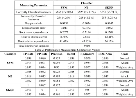
Table 2: Performance Measurement Comparison Values

Classifier TP Rate FP Rate Precision Recall F-Measure ROC Area Class

SVM

0.999 0.086 0.923 0.999 0.959 0.956 Normal 0.914 0.001 0.998 0.914 0.954 0.956 Attack 0.957 0.044 0.96 0.957 0.957 0.956 Weighted Avg

NB

0.985 0.082 0.925 0.985 0.954 0.958 Normal

0.918 0.015 0.983 0.918 0.949 0.947 Attack 0.952 0.049 0.954 0.952 0.952 0.953 Weighted Avg

SKNN

1 0.087 0.922 1 0.96 0.994 Normal

0.913 0 1 0.913 955 994 Attack

0.957 0.044 0.961 0.957 0.957 0.994 Weighted Avg

Simple k-nearest neighbor has recorded high accuracy SVM and NB classifiers. SKNN has achieved 95.71% of accuracy, on the other hand SVM and NB has recorded 95.70% and 95.17% of accuracy respectively.

5. CONCLUSION

Interruption discovery and avoidance are basic to present and future systems and data frameworks, on the grounds that our day by day exercises are vigorously reliant on them. Moreover, future difficulties will turn out to be all the more overwhelming due to the Internet of Things. In this admiration, interruption recognition frameworks have been essential over the most recent couple of decades. A few procedures have been utilized in interruption discovery frameworks, however machine learning methods are basic in late writing. Furthermore, extraordinary machine learning strategies have been utilized, however a few methods are increasingly appropriate for examining gigantic information for interruption recognition of system and data frameworks. To address this issue, diverse machine learning methods, specifically, SVM, NB, and SKNN are researched and looked at in this work.

REFERENCES

[1] H. Wang, J. Gu, S. Wang, An effective intrusion detection framework based on SVM with feature augmentation, Knowledge-Based Systems, Volume 136, 2017, Pages 130-139, ISSN 0950-7051, https://doi.org/10.1016/j.knosys.2017.09.0 14.

[2] F. Kuang, X. Weihong , S. Zhang, A novel hybrid KPCA and SVM with GA model for intrusion detection, Applied Soft Computing, Volume 18,2014,Pages 178-184,ISSN 1568-4946, https://doi.org/10.1016/j.asoc.2014.01.028 .

[3] A. A. Aburomman, M.B. Reaz, A novel SVM-kNN-PSO ensemble method for intrusion detection system, Applied Soft Computing, Volume 38, 2016, Pages 360-372, ISSN 1568-4946, https://doi.org/10.1016/j.asoc.2015.10.011 .

393 2017, Pages 1-12, ISSN 0950-7051,

https://doi.org/10.1016/j.knosys.2017.07.0 05.

[5] S. Teng, N. Wu, H. Zhu, L. Teng and W. Zhang, "SVM-DT-based adaptive and collaborative intrusion detection," in IEEE/CAA Journal of Automatica Sinica, vol. 5, no. 1, pp. 108-118, Jan. 2018. doi: 10.1109/JAS.2017.7510730.

[6] N.Farnaaz, M.A. Jabbar, Random Forest Modeling for Network Intrusion Detection System, Procedia Computer Science, Volume 89, 2016, Pages 213-217, ISSN 1877-0509,

https://doi.org/10.1016/j.procs.2016.06.04 7.

[7] R. M. Elbasiony, E.A. Sallam, T.E. Eltobely, M. M. Fahmy, A hybrid network intrusion detection framework based on random forests and weighted k-means, Ain Shams Engineering Journal, Volume 4, Issue 4,2013,Pages 753-762, ISSN 2090-4479,

https://doi.org/10.1016/j.asej.2013.01.003. [8] I.Ahmad, F. Amin, "Towards feature subset selection in intrusion detection," 2014 IEEE 7th Joint International Information Technology and Artificial Intelligence Conference, Chongqing, 2014, pp. 68-73.

[9] C.C .Chang,. and C.J. Lin., 2011. LIBSVM: a library for support vector machines. ACM transactions on intelligent systems and technology (TIST), 2(3), p.27.

[10]S.M. Bamakan, H. Wang, T. Yingjie, Y. Shi, An effective intrusion detection framework based on MCLP/SVM optimized by time-varying chaos particle swarm optimization, Neurocomputing, Volume 199, 2016, Pages 90-102.

[11]J.Jayshree, and L. Ragha. "Intrusion detection system using support vector machine." International Journal of Applied Information Systems (HAIS)-ISSN (2013): 2249-0868

[12]Y. Liu, Y. Wang, and J. Zhang, „New Machine Learning Algorithm: Random Forest‟, in Liu, B., Ma, M., and Chang, J. (Eds.): „Information Computing and Applications‟ (Springer Berlin Heidelberg, 2012), pp. 246-252

[13]G.B. Huang, Q.Y. Zhu and C.K. Siew, "Extreme learning machine: a new learning scheme of feedforward neural networks," 2004 IEEE International Joint Conference on Neural Networks (IEEE Cat. No.04CH37541), 2004, pp. 985-990 vol.2. doi: 10.1109/IJCNN.2004.1380068

[14]G. B. Huang, H. Zhou, X. Ding and R. Zhang, "Extreme Learning Machine for Regression and Multiclass Classification," in IEEE Transactions on Systems, Man, and Cybernetics, Part B (Cybernetics), vol. 42, no. 2, pp. 513-529, April 2012. doi: 10.1109/TSMCB.2011.2168604. [15]A. Qayyum, A.S. Malik, N.M.Iqbal, M.

Abdullah, M.F. Rasheed, W., Abdullah, T.A.R. and M.Y.B. Jafaar,., Image classification based on sparse-coded features using sparse coding technique for aerial imagery: a hybrid dictionary approach. Neural Computing and Applications,20017 pp.1-21. https://doi.org/10.1007/s00521-017-3300-5.

[16]A. Derhab, A. Bouras, M. R. Senouci, M. Imran, “Fortifying Intrusion detection systems in dynamic ad-hoc and wireless sensor networks”, International Journal of Distributed Sensor Networks, Vol. 2014. [17]I. Yaqoob, E. Ahmed, M. H. Rehman, A.

I. A. Ahmed, M. A. Al-Garadi, M. Imran, M. Guizani, The rise of ransomware and emerging security challenges and solutions in the Internet of Things, Computer Networks, Vol. 129, Part 2, pp. 444-458, Dec, 2017.