Distributed Optimization and Data Market Design

Thesis by

Palma London

In Partial Fulfillment of the Requirements for the degree of

Master of Science

CALIFORNIA INSTITUTE OF TECHNOLOGY Pasadena, California

2017

ACKNOWLEDGEMENTS

ABSTRACT

In this thesis we propose a new approach for distributed optimization based on an emerging area of theoretical computer science – local computation algo-rithms. The approach is fundamentally different from existing methodologies and provides a number of benefits, such as robustness to link failure and adap-tivity to dynamic settings. Specifically, we develop an algorithm, LOCO, that given a convex optimization problemP withn variables and a “sparse” linear constraint matrix with m constraints, provably finds a solution as good as that of the best online algorithm for P using only O(log(n+m)) messages with high probability. The approach is not iterative and communication is re-stricted to a localized neighborhood. In addition to analytic results, we show numerically that the performance improvements over classical approaches for distributed optimization are significant, e.g., it uses orders of magnitude less communication than ADMM.

PUBLISHED CONTENT AND CONTRIBUTIONS

Palma London, Niangjun Chen, Shai Vardi, and Adam Wierman. Distributed Optimization via Local Computation Algorithms. http://users.cms.caltech.

edu/~plondon/loco.pdf. Under submission. 2017.

P. London and S. Vardi came up with the results and proofs in this paper, and P. London coded and ran all experiments. Article adapted and extended for this thesis.

Xiaoqi Ren, Palma London, Juba Ziani, and Adam Wierman. Joint Data Pur-chasing and Data Placement in a Geo-Distributed Data Market. Proceedings of the 2016 ACM SIGMETRICS International Conference on Measurement and Modeling of Computer Science. 2016.

TABLE OF CONTENTS

Acknowledgements . . . iii

Abstract . . . iv

Table of Contents . . . vi

I Introduction and Motivation

1

II Distributed Optimization via Local Computation

Algorithms

4

2.1 Contributions of this work . . . 6

2.2 Related literature . . . 7

Chapter III: Network Utility Maximization . . . 9

3.1 Model . . . 9

3.2 Distributed Algorithms for Network Utility Maximization . . . 10

3.3 Performance metrics . . . 10

Chapter IV: Local Convex Optimization . . . 12

4.1 An overview of LOCO . . . 12

4.2 Analysis of LOCO . . . 15

4.3 Contrasting LOCO and ADMM . . . 17

Chapter V: Case Study . . . 18

5.1 Experimental setup . . . 18

5.2 Experimental Results . . . 21

Chapter VI: Concluding Remarks . . . 23

IIIData Purchasing and Data Placement in a

Geo-Distributed Data Market

24

Chapter VIII: Opportunities and challenges . . . 29

8.1 The potential of data markets . . . 29

8.2 Operational challenges for data markets . . . 30

Chapter IX: A Geo-Distributed Data Cloud . . . 33

9.1 Modeling Data Providers . . . 33

9.2 Modeling Clients . . . 34

9.3 Modeling a Geo-Distributed Data Cloud . . . 35

10.1 An exact solution for a single data center . . . 41

10.2 The design of

Datum

Chapter XI: Case Study . . . 49

11.1 Experimental setup . . . 49

11.2 Experimental results . . . 51

Chapter XII: Related work . . . 55

Chapter XIII: Conclusion . . . 57

Bibliography . . . 58

Appendix A: Pseudocode for General Online Fractional Packing . . . . 66

A.1 ADMM . . . 66

Appendix B: Proof of Lemma 3 . . . 68

Appendix C: Proof of Theorem 8 . . . 71

C.1 Proof of Theorem 9 . . . 72

C.2 Proof of Step 2 in §10.2 . . . 76

Part I

Introduction and Motivation

C h a p t e r 1

INTRODUCTION

We consider algorithms for distributed optimization and their applications. In this thesis we propose two new approaches to distributed optimization and consider an exciting application in distributed data markets.

The first algorithm, LOCO, is a fundamentally new approach to distributed optimization. There are a wide variety of approaches for distributed opti-mization, which fall into the categories of dual decomposition and subgradient methods, and consensus-based schemes. We propose a new approach which utilizes local computation algorithms, a rising field in theoretical computer science. A local algorithm is one where a query about part of a solution to a problem can be answered by communicating with only a small number of com-putation units in the distributed setting. Neither iterative descent methods nor consensus methods are local: answering a query about a part of the solu-tion requires global communicasolu-tion. The advantage offered by LOCO is that significantly less communication is required to solve the optimization problem [60].

Part II

Distributed Optimization via

Local Computation Algorithms

C h a p t e r 2

INTRODUCTION TO DISTRIBUTED OPTIMIZATION

The goal of this work is to introduce a new, fundamentally different approach to distributed optimization based on an emerging area of theoretical computer science – local computation algorithms.

Distributed optimization is an area of crucial importance to networked con-trol. Settings where multiple, distributed, cooperative agents need to solve an optimization problem to control a networked system are numerous and varied. Examples include management of content distribution networks and data cen-ters [13, 70], communication network protocol design [47, 62, 84], trajectory optimization [39, 53], formation control of vehicles [86, 75], sensor networks [69, 59], control of power systems [27, 72], and management of electric vehicles and distributed storage devices [16, 35].

Distributed optimization is a field with a long history. Beginning in the 1960s approaches emerged for solving large scale linear programs via decomposition into pieces that could be solved in a distributed manner. For example, two early approaches are Bender’s decomposition [9] and the Dantzig-Wolfe de-composition [24, 23], which can both be generalized to nonlinear objectives via the subgradient method [10, 67, 83].

Today, there is a wide variety of approaches for distributed optimization, e.g., primal decomposition [54, 10] and dual decomposition [28, 67, 61, 84]. See [71] for a survey. Broadly, these approaches tend to fall into two categories. The first category uses dual decomposition and subgradient methods [47, 61, 84]; the second involves consensus-based schemes which enable decentralized information aggregation, which forms the basis for many first order and second order distributed optimization algorithms [12, 66].

While the algorithms described above are distributed, they are not local. A local algorithm is one where a query about a small part of a solution to a problem can be answered by communicating with only a small neighborhood around the part queried1 _{(see Subsection 2.2 for a more comprehensive}

tion and example). Clearly, neither iterative descent methods nor consensus methods are local: answering a query about a piece of the solution requires global communication.

Local computation is well suited for distributed optimization. For example, any failure in the system only has local effects: if a node in a distributed system goes offline while an iterative distributed algorithm is executing, the whole process is brought to a halt (or at least the system needs to be carefully designed to be able to accommodate such failures); if the computations are all local, the failure will only affect a small number of nodes in the neighborhood of the failure. Similarly, lag in a single edge affects the computation of the entire solution in the iterative setting, while most computations are not be affected at all when the computations are local. Another advantage of local computation is that it allows the system to be more dynamic: an arrival of another node requires recomputing the entire solution if the algorithm is not local, but requires only a few local messages and computations if the algorithm is local.

Despite the benefits of local algorithms for distributed optimization, the prob-lem of designing a local, distributed optimization algorithm is open.

2.1 Contributions of this work

This paper introduces an algorithm, LOCO, (LOcal Convex Optimization) that is both distributed and local. It is not an iterative method and uses far less communication to compute small parts of the solution than iterative descent and consensus methods, e.g., ADMM and dual decomposition, while matching the total communication if the whole solution is queried.

While the technique we propose is general, in this work, we focus on a canoni-cal optimization problem: network utility maximization. Due to space restric-tions, we only consider the variant of maximizing throughput, which amounts to solving a distributed linear program. We focus on this case because it is par-ticularly well-studied and, in addition, the objective function is linear, which in many cases is known to produce the worst performance guarantee for online convex optimization problems [5, 41].

LOCO uses orders of magnitude less communication than ADMM if only part of the solution is required, and the same order of magnitude if the entire solution is required. Furthermore, in terms of both the amount of communica-tion required and the relative error, LOCO vastly outperforms its theoretical guarantees.

The key idea behind LOCO is an extension of recent results from the emerging field of local computation algorithms (LCA) in theoretical computer science (e.g., [63, 76, 56]). In particular, a key insight of the field is that online algorithms can be converted into local algorithms in graph problems with bounded degree [63]. However, much of the focus of local algorithms has, to this point, been on graph problems (see related literature below). The technical contribution of this work is the extension of these ideas to convex programs.

2.2 Related literature

This work, for the first time, brings techniques from the field of local com-putation algorithms into the domain of networked control. The LCA model was formally introduced by Rubinfeld et al. [78], after many algorithms fitting within the framework had recently appeared in distinct areas, e.g., [79, 4, 46]. LCAs have received increasing attention in the years that followed as the im-portance of local, distributed computing has grown with the increasing scale of problems in distributed systems, the internet of things, etc.

The main idea of LCAs is to compute a piece of the solution to some algorith-mic problem using only information that is close to that piece of the problem, as opposed to a global solution, by exchanging information across distributed agents. More concretely, an LCA receives a query and is expected to output the part of the solution associated with that query. For example, an LCA for maximal matching would receive as a query an edge, and its output would be “yes/no”, corresponding to whether or not the edge is part of the required matching. The two requirements are (i) the replies to all queries are consistent with the same solution, and (ii) the reply to each query is “efficient”, for some natural notion of efficient.

C h a p t e r 3

NETWORK UTILITY MAXIMIZATION

In order to illustrate the application of local computation algorithms to dis-tributed optimization, we focus on the classic setting of network utility maxi-mization (NUM). The NUM framework is a general class of optimaxi-mization prob-lems that has seen wide-spread application to distributed control in domains from the design of TCP congestion control [47, 61, 62, 84] to understanding of protocol layering as optimization decomposition [18, 71] and power system demand response [80, 58]. For a recent survey, see [96].

3.1 Model

The NUM framework considers a network containing a set of links L = {1, . . . , m} of capacity cj, for j ∈ L. A set of N = {1, . . . , n} sources shares

the network; source i ∈ N is characterized by (Li, fi, xi,x¯i): a path Li ⊆ L

in the network; a (usually) concave utility function fi : R+ → R; and the minimum and maximum transmission rates ofi.

The goal in NUM is to maximize the sources’ aggregate utility. Sourceiattains a concave utilityfi(xi) when it transmits at ratexi that satisfiesxi ≤xi ≤x¯i;

the optimization of aggregate utility can be formulated as follows,

max

x

n

X

i=1 fi(xi)

subject to Ax≤c x≤x≤x,¯

where A∈_Rm₊×n is defined as Aji =







1, j ∈L(i) 0, otherwise

.

The NUM framework is general in that the choice of fi allows for the

rep-resentation of different goals of the network operator. For example, using fi(xi) = xi, maximizes throughput; setting fi(xi) = log(xi) achieves

propor-tional fairness among the sources; setting fi(xi) =−1/xi minimizes potential

In this paper we focus on the throughput maximization case, i.e.,fi(xi) = xi; in

this case NUM is an LP. Note that the classical dual decomposition approach does not work for throughput maximization since it requires the objective function to be strictly concave. However, ADMM can be applied.

Our complexity results hinge on the assumption that the constraint matrix A is sparse. Thesparsity ofAis defined as max{α, β}, whereαandβ denote the maximum number of non-zero entries in a row and column of A respectively. Formally, we say thatAissparse if the sparsity ofAis bounded by a constant. This assumption usually holds in network control applications since α is the maximum number of sources sharing a link, which is typically small compared ton, andβis the maximum number of links each source uses, which is typically small compared tom.1

3.2 Distributed Algorithms for Network Utility Maximization

Given the NUM formulation above, the algorithmic goal is to design a protocol that efficiently finds an (approximately) optimal solution. If the network is huge, it is often beneficial to distribute the solution, as performing the entire computation on a single machine is too costly [14, 84].

There is a large literature across the networked control and communication networks literatures that seeks to design such distributed optimization al-gorithms, e.g., [18, 47, 62]. Dual decomposition algorithms are particularly prominent for use in this setting. However, many such methods cannot be applied to the case of throughput maximization, i.e., linearfi. One extremely

prominent algorithm that does apply in the case of throughput maximization is Alternating Method of Multipliers (ADMM), which was introduced by [34] and has found broad applications in e.g., denoising images [85], support vector machine [33], and signal processing [20, 19, 81]. As a result, we use ADMM as a benchmark for comparison in this paper. For completeness, the application of ADMM to NUM is described in Appendix A.1.

3.3 Performance metrics

Distributed algorithms for NUM should perform well on two measures. The first is message complexity: the number of messages that are sent across

1_{Whenαis large, many links will be congested and all sources will experience greater}

s1 s2 s3 t2 t₃ t1

e1 e2 _e

3 e4 e1 e2 e4 e₃

s₁ s₂ s₃

e₁ 1 0 0

e2 1 1 0

e3 0 1 1

e₄ 0 0 1

s₁ s₂ s3 e₁ e₂ e₃ e₄ 0.3 0.4 0.1 (a)

(b) (c) (d)

0.2

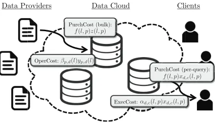
Figure 3.1: An illustration of LOCO on a toy graph with five nodes and four edges, e1, . . . , e4. There are three sources, s1, s2, s3, with paths ending in destinations t1, t2, t3 respectively. The graph is depicted in (a); the constraint matrix for NUM is given in (b); the bipartite graph representation of the matrix in (c); and the dependency graph in (d). The rank of each constraint (edge) is written in the node representing the constraint in the dependency graph. The shaded nodes represent the query set for sources1.

links of the network in order to compute the solution. When the algorithm uses randomization, we want the message complexity to hold with probability at least 1− 1

nα, where where n is the number of vertices in the network and

α >0 can be an arbitrarily large constant. We denote this by 1− 1

polyn. We

do not bound the size of the messages, but note that in both our algorithm and ADMM the message length will be of order O(logn).

C h a p t e r 4

LOCAL CONVEX OPTIMIZATION

In this section, we introduce a local algorithm for distributed convex opti-mization,LOcal Convex Optimization (LOCO). In LOCO, every source in the network computes its portion of a near optimal solution using a small number of messages, without needing global communication or iteration. This is in contrast to iterative descent methods, e.g. ADMM, which areglobal, i.e., they spread the information necessary to find an optimal solution throughout the whole network over a series of rounds. LOCO has provable worst-case guaran-tees on both its approximation ratio and message complexity, and improves on the communication overhead of iterative descent methods by orders of magni-tude in practice when asked to compute a piece of the optimal solution.

4.1 An overview of LOCO

The key insight in the design and analysis of LOCO is that any natural1 _online optimization algorithm can be converted into a local, distributed optimization algorithm. Note that the resulting distributed algorithm is for a static problem, not an online one. Further, after this conversion, the distributed optimization algorithm has the same approximation ratio as the original online optimization algorithm. Thus, given an optimization problem for which there exist effective online algorithms, these online algorithms can be converted into effective local, distributed algorithms.

More formally, to reduce a static optimization problem to an online optimiza-tion problem, we do the following. LetY be the set of constraints of an opti-mization problemP. Letr :Y →[0,1] be a ranking function that assigns each constraint yj a real number between 0 and 1, uniformly at random. We call

r(yj)yj’srank. Suppose that there is some online algorithmALGthat receives

the constraints sequentially and must augment the variables immediately and

1_{Strictly speaking, we require that the online algorithm have the following characteristic:}

knowing the output of the algorithm for the “neighbors” of a queryq that arrived before

irrevocably so as to satisfy each arriving constraint. Suppose furthermore that for each constraint yj, we can pinpoint a small set of constraints S(yj) (which

we call yj’s query set) that arrived before it so that restricting the set of

con-straints ofP toS(yj) results inALGproducing (exactly) the same solution for

the variables that are present inyj. Then simulatingALGonly onS(yj) would

suffice to obtain the solution for the variables inyj. This is precisely what our

algorithm does: it generates a random order of arrival for the constraints, and for each constraint yj, it constructs such a set S(yj) and simulates the online

algorithm on it. An arbitrary ordering could mean that these dependency sets are very large for some constraints; to bound the size of these sets, we require that (i) the constraint matrix of P is sparse and (ii) the order generated is random.2

Concretely, there are two main steps in LOCO. In the first, LOCO generates a localized neighborhood for each vertex. In the second, LOCO simulates an online algorithm on the localized neighborhood. Importantly, the first step is independent of the precise nature of the online algorithm, and the second is independent of the method used to generate the localized neighborhoods. Therefore, we can think of LOCO as a general methodology that can yield a variety of algorithms. For example, we can use different online algorithms for the second step of LOCO depending on whether we consider a linear NUM problem or a strictly convex NUM problem. More specifically, the two steps work as follows.

Step 1, Generating a localized neighborhood For clarity, we break the first step into three sub-steps, see also Figure 3.1.

Step 1a, Representing the constraint matrix as a bipartite graph A boolean matrix A can be represented as a bipartite graph G = (L, R, E0) as follows. Each row of A is represented by a vertex v` ∈ L; each column by

a vertex vr ∈ R. The edge (v`, vr) is in E0 if and only if A`,r = 1. A more

intuitive way to interpret G is the following: L represents the variables, R the constraints. Edges represent which variables appear in which constraints. Note that the maximum degree of G is exactly the sparsity of A.

Step 1b, Constructing the dependency graph We construct the depen-dency graph H = (V, E) as follows. The vertices of the dependency graph are the vertices of R; an edge exists between two vertices in H if the corre-sponding vertices in Gshare a neighbor. Intuitively, H represents the “direct dependencies” between the constraints: changing the value of any variable im-mediately affects all constraints in which it appears, hence these constraints can be thought of as directly dependent. The maximum degree ofH is upper bounded by the square of the sparsity of A.

Step 1c, Constructing the query set In order to build the query set, we generate a randomranking function on the vertices ofH,r :V →[0,1]. Given the dependency graph H, an initial node y ∈ V and the ranking function r, we build the query set ofy, denotedS(y), using a variation of BFS, as follows. InitializeS(y) to containy. For every vertexv ∈S(y), scan all ofv’s neighbors, denoted N(v). For each u ∈ N(v), if r(u) ≤ r(v), add u to S(y). Continue iteratively until no more vertices can be added toS(y) (that is, for every vertex v ∈S(y) all of its neighbors that are not themselves in S(y) have lower rank than v). If there are ties (i.e., two neighbors u, v such that r(u) =r(v)), we tie-break by ID.3

Step 2, Simulating the online algorithm Assume that we have an online algorithm for the problem that we would like LOCO to solve (in this paper we use the online packing Algorithm of Buchbinder and Naor [15, chapter 14]. We provide the pseudocode in Appendix A, for completeness). The specific setting that the online algorithm must apply to is the following: the variables of the convex program are known in advance, as are the univariate constraints. The (rest of the) constraints arrive one at a time; the online algorithm is expected to satisfy each constraint as it arrives, by increasing the value of some of the variables. It is never allowed to decrease the value of any variable. We simulate the online algorithm as follows:

In order to compute its own value in the solution, source i applies r to the set of constraints in which it is contained, Y(i). For y= arg max_z∈Y(i){r(z)}, it simulates the online algorithm on S(y). That is, it executes the online algorithm on the neighborhood constructed in Step 1 for the “last arriving”

constraint that contains i. i’s value is the value ofi at the end of the simula-tion. Claim 4 below shows that i’s value is identical to its value if the online algorithm was executed on the entire program, with the constraints arriving in the order defined byr.

4.2 Analysis of LOCO

Our main theoretical result shows that LOCO can compute solutions to convex optimization problems that are as good as those of the best online algorithms for the problems using very little communication. We then specialize this case to throughput maximization in NUM. While we focus on NUM in this paper, the theorem (and its proof) apply to a wider family of problems as well. Specifically, the conversion from online to local outlined below can be used more broadly for any class of optimization problems for which effective online algorithms exist. Thus, improvements to online optimization problems immediately yield improved local optimization algorithms.

Theorem 1 Let P be a problem with a concave objective function and linear inequality constraints, with n variables and m constraints, whose constraint matrix has sparsity σ. Given an online algorithm4 for P with competitive ratio h(n, m), there exists a local computation algorithm for P with approx-imation ratio h(n, m) that uses 2O(σ2₎

log (n+m) messages with probability 1−1/poly(n, m).

In particular, we have the following result, for NUM with a linear objective function.

Theorem 2 Let P be a throughput maximization problem with n variables, m constraints, and a sparse constraint matrix. LOCO computes an O(logm) – approximation to the optimal solution of P usingO(log(n+m))messages with probability 1−1/poly(n, m).

The approximation ratio in Theorem 2 comes from the online algorithm pre-sented and analyzed in [15] (see Lemma 6). The analysis of the online al-gorithm is for adversarial input; therefore it is natural to expect LOCO to achieve a much better approximation ratio in practice, as LOCO randomizes

the order in which the constraints “arrive”. It is an open question to give bet-ter theoretical bounds for stochastic inputs, and if such results are obtained they would immediately improve the bounds in Theorem 2.

The core technical lemma required for the proof of Theorem 1 is the following.

Lemma 3 Let G = (V, E) be a graph whose degree is bounded by d and let r:V →[0,1]be a function that assigns to each vertexv ∈V a number between 0 and 1 independently and uniformly at random. Let Tmax be the size of the

largest query set of G: Tmax = max{|Tv|:v ∈V}. Then, for λ= 4(d+ 1),

Pr[|Tmax|>2λ·15λlogn]≤

1 n2.

The proof of Lemma 3 uses ideas from a proof in [76], and employs a quantiza-tion of the rank function. Its proof is deferred to Appendix B. The following simple claim implies that the approximation ratio of LOCO is the same as that of the online algorithm.

In addition to Lemma 3, the following claim and technical lemma are needed to complete the proof of Theorem 2.

Claim 4 For any source i, the value of xi in the output of LOCO is identical

to its value in the output of the online algorithm.

Proof 5 Let constraint yj be the last constraint containing i that arrives in

the order defined by r; its arrival is the last time iwill be updated. Therefore it is sufficient to only consider constraints arriving before yj. Further, by design,

S(yj) is the set of constraints at whose arrival there is possibly some change

that may affect the value of i.

The following lemma is a restatement of Theorem 14.1 in [15], adapted to throughput maximization. See Appendix A for the pseudocode of the algo-rithm.

Lemma 6 For any B >0, there exists is a B-competitive online algorithm to linearly-constrained NUM with m constraints; each constraint is violated by a factor at most 2 log(1+_B m).

4.3 Contrasting LOCO and ADMM

LOCO fundamentally differs from iterative descent and consensus style ap-proaches to distributed optimization. While iterative descent and consensus style approaches are inherently iterative, LOCO is not. Under LOCO, a node can compute its value in one shot, once it gets information about its query set. Additionally, while iterative descent and consensus style approaches areglobal, LOCO is local. Under LOCO, communication stays within the query set and so the computation only needs to be updated if changes happen within the query set. This means that LOCO is robust to churn, failures, and communication problems outside of that set of nodes.

Another important difference is that LOCO does not compute the optimal so-lution, while iterative descent and consensus style approaches will eventually converge to the true optimal. The proven analytical bounds for LOCO are based on worst-case adversarial input. We show in Section 5.2 that our em-pirical results outperform the theoretical guarantees by a considerable margin. This is in part because the ranking is done randomly rather than in an adver-sarial fashion (we elaborate on this in Section 5).

C h a p t e r 5

CASE STUDY

Here we present the results of a simulation study demonstrating the empirical performance of LOCO on both synthetic and real networks. The results high-light that an orders-of-magnitude reduction in communication is possible with LOCO as compared to ADMM, which we choose as a prominent example of current approaches for distributed optimization. For concreteness, our exper-iments focus our numeric results on distributed linear programming, i.e., the case of linear NUM. This is the NUM setting where one could expect LOCO to perform the worst, given that linear functions are typically the worst-case examples for online convex optimization algorithms [5, 41].

5.1 Experimental setup Problem Instances

For our first set of experiments, we generate random synthetic instances of linear NUM. Let n = m and define the constraint matrix A ∈ _R(m×n) _as follows. Set ˜Aj,i = 1 with probabilitypand ˜Aj,i= 0 otherwise. Let A= ˜A+In

to ensure each row ofA has at least one non zero entry.1 _{The vector c∈}

Rn is

drawn i.i.d.from Unif[0,1]. We set the minimum and maximum transmission rates to be x_i = 0 and ¯xi = 1. Finally, for the rank function used by LOCO

we use a random permutation of the vertex IDs.2

For our second set of experiments, we use the real network from the graph of Autonomous System (AS) relationships in [87]. The graph has 8020 nodes and 36406 edges. In order to interpret the graph in a NUM framework, we associate each source with a path of links, ending at a destination node. To do this, for each nodeiin the graph, we randomly select a destination node ti

which is at distance `i, sampled i.i.d. from Unif[`−0.5`, `+ 0.5`]. We repeat

this for several values of `. (The distance between two nodes is the length

1_{Note that this matrix does not have constant sparsity; however this can only increase}

the message complexity. Irregardless, it is possible to adapt the theoretical results to hold for this data as well, using techniques from [76].

2_{For the purposes of our simulations, such a permutation can be efficiently sampled, and}

0 5000 10000 15000 0

5 10 15x 10

6 n Messages ADMM 1 ADMM 2 LOCO Tot LOCO Max LOCO Avg (a)

0 5000 10000 15000

100 102 104 106 108 n Messages ADMM 1 ADMM 2 LOCO Tot LOCO Max LOCO Avg (b)

1 1.5 2

x 10−4 0

4 8 12x 10

6 p Messages ADMM 1 ADMM 2 LOCO Tot LOCO Max LOCO Avg (c)

0.5 1 1.5 2

x 10−4 100 102 104 106 108 p Messages ADMM 1 ADMM 2 LOCO Tot LOCO Max LOCO Avg (d)

Figure 5.1: Illustration of the number of messages required by ADMM and LOCO for the synthetic data set with results averaged over 50 trials. Plots (a) and (b) vary n while fixing sparsity p = 10−4_{, showing the results in} linear-scale and log-linear-scale respectively. Plots (c) and (d) fix n = 103 and vary the sparsity p, showing the results in linear-scale and log-scale respectively.

of the shortest path between them.) Then, we designate the path L(i) to be the set of links comprising the shortest path between the source and the destination. The vectors c, x,and ¯xare chosen in the same manner as for the synthetic networks.

Algorithm tuning

Our results focus on comparing LOCO and ADMM. Running ADMM requires tuning four parameters [14]. Unless otherwise specified, we set the relative and absolute tolerances to berel = 10−4andabs = 10−2, the penalty parameter to be ρ= 1, and the maximum number of allowed iterations to betmax = 10000.

This is done to provide the best performance for ADMM: the parameters are tuned in the typical fashion to optimize ADMM [14]. Running LOCO requires tuning only one parameter: B, which governs the worst-case guarantee for the online algorithm used in step 2. A smaller B gives a “better guarantee”, however some constraints may be violated. Setting B = 2 ln(1 +m) provides the best worst-case guarantee, and is our choice in the experiments unless stated otherwise. In fact, it is possible to tune B (akin to tuning ADMM) to specific data, as the constraints are often still satisfied for smaller B. In Figure 5.3 (c), we show the improvement in performance guarantee by tuning B, while keeping the dual solution feasible.

Metrics

5 10 15 20 0

2 4 6

8x 10

6

Average Path Length

Messages ADMM LOCO Tot LOCO Max LOCO Avg (a)

5 10 15 20

100

105

1010

Average Path Length

Messages ADMM LOCO Tot LOCO Max LOCO Avg (b)

Figure 5.2: Illustration of the number of messages required by ADMM and LOCO for the real network data with n = 8020 and various average path lengths L(i).

0 0.05 0.1 0.15 0.2 103 104 105 106 107 Relative Error Messages ADMM LOCO Tot LOCO Max LOCO Avg (a)

0 0.05 0.1 0.15 0.2 103 104 105 106 107 Relative Error Messages ADMM LOCO Tot LOCO Max LOCO Avg (b)

10 11 12 13 14 0 0.05 0.1 0.15 0.2 0.25 B Relative Error LOCO (c)

Figure 5.3: Comparison of the relative error and the number of messages required by LOCO and ADMM. Plots (a) and (b) show the Pareto optimal curve for ADMM with a range of relative tolerances rel _{∈ {10}−4_,10−1_{}. Plot} (c) depicts how tuning B effects the relative error. The right most point corresponds to B = 2 ln(1 +m).

To assess the quality of the solution we measure the relative error, which is defined as |p∗−_|p_pLOCO∗_| |, wherep∗ is the optimal solution. For problem instances

of small dimension, one can run an interior point method to check the optimal solution, but this is too tedious for large problem sizes. In the large dimension cases we consider, we regardp∗ to be ADMM’s solution with small tolerances, such that the maximum number of allowed iterations is never needed. Note that the relative error is an empirical, normalized version of the approximation ratio for a given instance.

is proportional to the number of edges with at least one endpoint in the query set (this is the number of edges we need to send information over in order to construct the query set, see e.g., [76] for more details). We note that the number of messages depends both on the network topology and the realization of the ranking function.

5.2 Experimental Results

We now describe our empirical comparison of the performance of LOCO with ADMM.

Our first set of experiments investigates the communication used by ADMM and LOCO, i.e., the number of messages required. Figure 5.1 highlights that LOCO requires considerably fewer messages than ADMM, across both small and large n and varying levels of sparsity. More specifically, the figure shows that both the average and maximum amount of communication needed to answer a query about a specific piece of the solution under LOCO (LOCO Avg and LOCO Max respectively) are substantially lower than for ADMM. Further, even answeringevery query (LOCO Tot) requires only the same order of magnitude as ADMM. The figure includes ADMM with a tolerance rel of 10−4 _{(ADMM 1) and 10}−3 _{(ADMM 2). Even with suboptimal tolerance,} which results in fewer iterations, ADMM still requires orders of magnitude more communication than LOCO.

Figure 5.2 shows the same qualitative behavior in the case of the real network data. In particular, the number of messages used is shown as a function of the average length of paths in the AS topology. We see that LOCO greatly outperforms ADMM for all tested average path lengths.

The improvement achieved by LOCO is possible because the size of the query sets used by LOCO are small compared to the number of sources. When n = 103_{, as in Figure 5.1, the number of nodes in the largest query set (over} all trials) was 60.

We note that the improvement in the amount of communication is achieved at a cost: LOCO does not precisely solve the optimization, it only approximates the solution. When B is set to its worst-case guarantee (Figure 5.1), the relative error of LOCO ranges from 0.29 to 0.34.

C h a p t e r 6

CONCLUDING REMARKS

We introduced a new, fundamentally different approach for distributed opti-mization based on techniques from the field of local computation algorithms. In particular, we designed a generic algorithm, LOCO, that constructs small neighborhoods and simulates an online algorithm on them. Due to the fact that LOCO is local, it has several advantages over existing methods for dis-tributed optimization. In particular, it is more robust to network failures, communication lag, and changes in the system. To illustrate the benefits of LOCO we considered throughput maximization. The improvements of LOCO over ADMM in terms of communication in this setting are significant.

Part III

Data Purchasing and Data

Placement in a Geo-Distributed

Data Market

C h a p t e r 7

INTRODUCTION TO DISTRIBUTED DATA MARKETS

Ten years ago computing infrastructure was acommodity – the key bottleneck for new tech startups was the cost of acquiring and scaling computational power as they grew. Now, computing power and memory are services that can be cheaply subscribed to and scaled as needed via cloud providers like Amazon EC2, Microsoft Azure, etc.

We are beginning the same transition with respect to data. Data is broadly being gathered, bought, and sold in various marketplaces. However, it is still a commodity, often obtained through offline negotiations between providers and companies. Thus, acquiring data is one of the key bottlenecks for new tech startups nowadays.

This is beginning to change with the emergence of cloud data markets, which offer a single, logically centralized point for buying and selling data. Multiple data markets have recently emerged in the cloud, e.g., Microsoft Azure Data-Market [65], Factual [29], InfoChimps [44], Xignite [95], IUPHAR [88], etc. These marketplaces enable data providers to sell and upload data and clients to request data from multiple providers (often for a fee) through a unified query interface. They provide a variety of services: (i) aggregation of data from multiple sources, (ii) cleaning of data to ensure quality across sources, (iii) ease of use, through a unified API, and (iv) low-latency delivery through a geographically distributed content distribution network.

precision/quality and privacy may be a concern.

Not surprisingly, the design of pricing (both on the client side and the data provider side) has received significant attention in recent years, including pric-ing of per-query access [49, 51] and pricpric-ing of private data [32, 57].

In contrast, the focus of this paper isnot on the design of pricing strategies for data markets. Instead, we focus on the engineering side of the design of a data market, which has been ignored to this point. Supposing that prices are given, there are important challenges that remain for the operation of a data market. Specifically, two crucial challenges relate todata purchasing and data placement.

Data purchasing: Given prices and contracts offered by data providers, which providers should a data market purchase from to satisfy a set of client queries with minimal cost?

Data placement: How should purchased data be stored and replicated through-out a geo-distributed data market in order to minimize bandwidth and latency costs? And which clients should be served from which replicas given the loca-tions and data requirements of the clients?

Clearly, these two challenges are highly related: data placement decisions de-pend on which data is purchased from where, so the bandwidth and latency costs incurred because of data placement must be balanced against the pur-chasing costs. Concretely, less expensive data that results in larger bandwidth and latency costs is not desirable.

Thus, the design of a geo-distributed data market necessitates integrating data purchasing decisions into a geo-distributed data analytics system. To that end, our design builds on the model used in [92] by adding data providers that offer a menu of data quality levels for differing fees. The data placement/replication problem in [92] is already an integer linear program (ILP), and so it is no surprise that the addition of data providers makes the task of jointly optimizing data purchasing and data placement NP-hard (see Theorem 8).

Consequently, we focus on identifying structure in the problem that can allow for a practical and near-optimal system design. To that end, we show that the task of jointly optimizing data purchasing and data placement is equivalent to the uncapacitated facility location problem (UFLP) [52]. However, while constant-factor polynomial running time approximation algorithms are known for the metric uncapacitated facility location problem (see [17, 38, 45]), our problem is anon-metric facility location problem, and the best known polyno-mial running time algorithms achieve aO(logC) approximation via the greedy algorithm in [42] or the randomized rounding algorithm in [90], where C is the number of clients. Note that without any additional information on the costs, this approximation ratio is the smallest achievable for the non-metric uncapacitated facility location unless NP has slightly superpolynomial time algorithms [30]. While this is the best theoretical guarantee possible in the worst-case, some promising heuristics have been proposed for the non-metric case, e.g., [26, 8, 1, 48, 89, 36].

Though the task of jointly optimizing data purchasing and data placement is computationally hard in the worst case, in practical settings there is structure that can be exploited. In particular, we provide an algorithm with polynomial running time that gives an exact solution in the case of a data market with a single data center (§10.1). Then, using this structure, we generalize to the case of a geo-distributed data cloud and provide an algorithm, namedDatum(§10.2) that is near optimal in practical settings.

the data market). This decomposition is of crucial operational importance because it means that internal placement and routing decisions can proceed without factoring in data purchasing costs, mimicking operational structures of geo-distributed analytics systems today.

We provide a case study in §11 which highlights that Datum is near-optimal (within 1.6%) in practical settings. Further, the performance of Datum im-proves upon approaches that neglect data purchasing decisions by >45%. To summarize, this paper makes the following main contributions:

1. We initiate the study of jointly optimizing data purchasing and data place-ment decisions in geo-distributed data markets.

2. We prove that the task of jointly optimizing data purchasing and data placement decisions is NP-hard and can be equivalently viewed as a facility location problem.

3. We provide an exact algorithm with polynomial running time for the case of a data market with a single data center.

C h a p t e r 8

OPPORTUNITIES AND CHALLENGES

Data is now a traded commodity. It is being bought and sold every day, but most of these transactions still happen offline through direct negotiations for bulk purchases. This is beginning to change with the emergence of cloud data markets such as Microsoft Azure DataMarket in [65], Factual [29], In-foChimps [44], Xignite [95]. As cloud data markets become more prominent, data will become a service that can be acquired and scaled seamlessly, on demand, similarly to computing resources available today in the cloud.

8.1 The potential of data markets

The emergence of cloud data markets has the potential to be a significant disruptor for the tech industry, and beyond. Today, since computing resources can be easily obtained and scaled through cloud services, data acquisition has become the bottleneck for new tech startups.

For example, consider an emerging potential competitor for Yelp. The biggest development challenge is not algorithmic or computational. Instead, it is ob-taining and managing high quality data at scale. The existence of a data market, e.g., Azure DataMarket, with detailed local information about re-straints, attractions, etc., would eliminate this bottleneck entirely. In fact, data markets such as Factual [29] are emerging to target exactly this need. Another example highlighted in [50, 51] is language translation. Emerging data markets such as the Azure DataMarket and Infochimps sell access to data on word translation, word frequency, etc. across languages. This access is a crucial tool for easing the transition tech startups face when moving into different cultural markets.

Thus, like in the case of cloud computing, ease of access and scaling, combined with the cost efficiency that comes with size, implies that cloud data markets have the potential to eliminate one of the major bottlenecks for tech startups today – data acquisition.

8.2 Operational challenges for data markets

The task of designing a cloud data market is complex, and requires balancing economic and engineering issues. It must carefully consider purchasing and pricing decisions in its interactions with both data providers and clients and minimize its operational cost, e.g., from bandwidth. We discuss both the economic and engineering design challenges below, though this paper focuses only on the engineering challenges.

Pricing

While there is a large body of literature on selling physical goods, the problem of pricing digital goods, such as data, is very different. Producing physical goods usually has a moderate fixed cost, for example, for buying the space and production machines needed, but this cost is partly recoverable: it is possible, if the company cannot manage to sell its product, to resell the machinery and buildings they have been using. However, the cost of producing and acquiring data is high and irrecoverable: if the data turns out to be worthless and nobody wants it, then the whole procedure is wasted. Another major difference comes from the fact that variable costs for data are low: once it has been produced, data can be cheaply copied and replicated.

These differences lead to “versioning” as the most typical approach for selling digital goods [7]. Versioning refers to selling different versions of the same digital good at different prices in order to target different types of buyers. This pricing model is common in the tech industry, e.g., companies like Dropbox sell digital space at different prices depending on how much space customers need and streaming websites such as Amazon often charge differently for streaming movies at different quality levels.

suggested it is desirable to charge based on the complexity of the query, e.g., [6, 7]. Another form of versioning that has been proposed in data markets deals with privacy – data with more personal information should be charged more, e.g., [57, 22].

There is a growing literature focused on the design of pricing strategies for cloud data markets in the above, and other contexts, e.g., [6, 49, 7, 51, 7, 57, 22].

Data purchasing and data placement

While data pricing within cloud data markets has received increasing attention, the engineering of the system itself has been ignored. The engineering of such a geo-distributed “data cloud” is complex. In particular, the system must jointly make both data purchasing decisions and data placement, replication and delivery decisions, as described in the introduction.

worth it to place that data in data center A rather than data center B. In practice, the problem is more complex since clients are usually geo-graphically distributed rather than centralized and one client may require data from sev-eral different data providers.

C h a p t e r 9

A GEO-DISTRIBUTED DATA CLOUD

This paper presents a design for a geo-distributed cloud data market, which we refer to as a “data cloud.” This data cloud serves as an intermediary be-tweendata providers, which gather data and offer it for sale, andclients, which interact with the data cloud through queries for particular subsets/qualities of data. More concretely, the data cloud purchases data from multiple data providers, aggregates it, cleans it, stores it (across multiple geographically dis-tributed data centers), and delivers it (with low-latency) to clients in response to queries, while aiming at minimizing theoperational cost constituted of both bandwidth and data purchasing costs.

Our design builds on and extends the contributions of recent papers – specif-ically [92, 73] – that have focused on building geo-distributed data analytic systems but assume the data is already owned by the system and focus solely on the interaction between a data cloud and its clients. Unfortunately, as we highlight in §10, the inclusion of data providers means that the data cloud’s goal of cost minimization can be viewed as a non-metric uncapacitated facility location problem, which is NP-hard.

For reference, Figure 9.1 provides an overview of the interaction between these three parties as well as some basic notations.

9.1 Modeling Data Providers

The interaction between the data cloud and data providers is a key distinction between the setting we consider and previous work on geo-distributed data analytics systems such as [73, 92]. We assume that each data provider offers distinct data to the data cloud, and that the data cloud is a price-taker, i.e., cannot impact the prices offered by data providers. Thus, we can summarize the interaction of a data provider with the data cloud through an exogenous menu of data qualities and corresponding prices.

be {street address, zip code, city, county, state}. For numerical data, quality could take many forms, e.g., the numerical precision, the statistical precision (e.g., the confidence of an estimator), or the level of noise added to the data.1 Concretely, we consider a setting where there are P data providers selling different data, p ∈ P = {1,2, . . . , P}.2 _{Each data provider offers a set of} quality levels, indexed by l ∈ L = {1,2, . . . , Lp}, where Lp is the number of

levels that data provider p offers. We use q(l, p) to denote the data quality level l, offered by data provider p. Similarly, we use f(l, p) to denote the fee charged by data provider pfor data of quality level l. Importantly, the prices vary across providers p since different providers have different procurement costs for different qualities and different data.

The data purchasing contract between data providers and data cloud may have a variety of different types. For example, a data cloud may pay data provider based on usage, i.e., per query, or a data cloud may buy the data in bulk in advance. In this paper, we discuss both per-query data contracting and bulk data contracting. See §9.3 for details.

9.2 Modeling Clients

Clients interact with the data cloud through queries, which may require data (with varying quality levels) from multiple data providers.

Concretely, we consider a setting where there areCclients,c∈ C ={1,2, . . . , C}. A client c sends a query to the data center, requesting particular data from multiple data providers.3 _{Denote the set of data providers required by the} re-quest from client query c byG(c). The client query also specifies a minimum desired quality level,wc(p), for each data providerpit requests, i.e.,∀p∈G(c).

We assume that the client is satisfied with data at a quality level higher than or equal to the level requested.

More general models of queries are possible, e.g., by including a DAG modeling the structure of the query and query execution planning (see [92] for details). For ease of exposition, we do not include such detailed structure here, but it

1_{A common suggestion for guaranteeing privacy is to add Laplace noise to data provided}

to data markets, see e.g., [25, 57]

2_{We distinguish data providers based on data, i.e., one data provider sells multiple data}

is treated as multiple data providers.

3_{We distinguish clients based on queries, i.e., one client sends multiple queries is treated}

can be added at the expense of more complicated notation.

Depending on the situation, the client may or may not be expected to pay the data cloud for access. If the clients are internal to the company running the data cloud, client payments are unnecessary. However, in many situations the client is expected to pay the data cloud for access to the data. There are many different types of payment structures that could be considered. Broadly, these fall into two categories: (i) subscription-based (e.g., Azure DataMarket [65]) or (ii) per-query-based (e.g. Infochimps [44]).

In this paper, we do not focus on (or model) the design of payment structure between the clients and the data cloud. Instead, we focus on the operational task of minimizing the cost of the data cloud operation (i.e., bandwidth and data purchasing costs). This focus is motivated by the fact that minimizing the operation costs improves the profit of the data cloud regardless of how clients are charged. Interested readers can find analyses of the design of client pricing strategies in [49, 51, 57].

9.3 Modeling a Geo-Distributed Data Cloud

The role of the data cloud in this marketplace is as an aggregator and in-termediary. We model the data cloud as a geographically distributed cloud consisting of D data centers, d∈ D ={1,2, . . . , D}. Each data center aggre-gates data from geographically separate local data providers, and data from data providers may be (and often is) replicated across multiple data centers within the data cloud.

Note that, even for the same data with the same quality, data transfer from the data providers to the data cloud is not a one time event due to the need of the data providers to update the data over time. We target the modeling and optimization of data cloud within a fixed time horizon, given the assumption that queries from clients are known beforehand or can be predicted accurately. This assumption is consistent with previous work [92, 73] and reports from other organizations [94, 55]. Online versions of the problem are also of interest, but are not the focus of this paper.

Modeling costs

or-Data Providers! Data Cloud! Clients!

OperCost: !

ExecCost: !αd,c(l, p)xd,c(l, p)

βp,d(l)yp,d(l)

PurchCost (bulk): !

! f(l, p)z(l, p)

PurchCost (per-query): !

! f(l, p)xd,c(l, p)

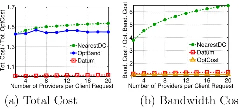
Figure 9.1: An overview of the interaction between data providers, the data cloud, and clients. The dotted line encircling the data centers (DC) represents the geo-distributed data cloud. Data providers and clients interact only with the cloud. Data provider p sends data of quality q(l, p) to data center d, and the corresponding operation cost is βp,d(l)yp,d(l). Similarly, data center d

sends data of qualityq(l, p) to clientc, and the corresponding execution cost is αd,c(l, p)xd,c(l, p). In bulk data contracting, the corresponding purchasing cost

is f(l, p)z(l, p). In per-query data contracting, the corresponding purchasing cost is f(l, p)xd,c(l, p).

der to describe these costs, we use the following notation, which is summarized in Figure 9.1.4

xd,c(l, p)∈ {0,1}: xd,c(l, p) = 1 if and only if data of qualityq(l, p), originating

from data provider p, is transferred from data centerd to client c. αd,c(l, p): cost (including bandwidth and/or latency) to transfer data of

qual-ityq(l, p), originating from data providerp, from data centerdto client c

yp,d(l) ∈ {0,1}: yp,d(l) = 1 if and only if data of quality q(l, p) is transferred

from data provider p to data centerd.

βp,d(l): cost (including bandwidth and/or latency) to transfer data of quality

q(l, p) from data providerp to data center d.

z(l, p) ∈ {0,1}: z(l, p) = 1 if and only if data of quality q(l, p), originating from data provider p, is transferred to the data cloud.

4_{Throughout, subscript indices refer to data transfer “from, to” a location, and}

f(l, p): purchasing cost of data with quality q(l, p), originating from data provider p.

Given the above notations, the costs of the data cloud can be broken into three categories:

(i) The operation cost due to transferring data of all quality levels from data providers to data centers is

OperCost = P X p=1 Lp X l=1 D X d=1

βp,d(l)yp,d(l). (9.1)

(ii) The execution cost due to transferring data of all quality levels from data centers to clients is

ExecCost =

C

X

c=1

X

p∈G(c)

Lp X l=1 D X d=1

αd,c(l, p)xd,c(l, p). (9.2)

(iii) The purchasing cost (PurchCost) due to buying data from the data provider could result from a variety of differing contract styles. In this paper we consider two extreme options: per-query and bulk data con-tracting. These are the most commonly adopted strategies for data purchasing today.

In per-query data contracting, the data provider charges the data cloud a fixed rate for each query that uses the data provided by the data provider. So, if the same data is used for two different queries, then the data cloud pays the data provider twice. Given a per-query fee f(l, p) for data q(l, p), the total purchasing cost is

PurchCost(query) =

C

X

c=1

X

p∈G(c)

Lp X l=1 D X d=1

f(l, p)xd,c(l, p). (9.3)

In bulk data contracting, the data cloud purchases the data in bulk and then can distribute it without owing future payments to the data provider. Given a one-time fee f(l, p) for dataq(l, p), the total purchas-ing cost is

PurchCost(bulk) = P X p=1 Lp X l=1

To keep the presentation of the paper simple, we focus on the per-query data contracting model throughout the body of the paper and discuss the bulk data contracting model (which is simpler) in Appendix C.3.

Cost Optimization

Given the cost models described above, we can now represent the goal of the data cloud via the following integer linear program (ILP), where OperCost, ExecCost, and PurchCost are as described in equations (9.1), (9.2) and (9.3), respectively.

min

x,y OperCost + ExecCost + PurchCost (9.5)

subject to xd,c(l, p)≤yp,d(l)∀c, p, l, d (9.5a) Lp

X

l=1

D

X

d=1

xd,c(l, p) = 1, ∀c, p∈G(c) (9.5b) Lp

X

l=1

D

X

d=1

xd,c(l, p)q(l, p)≥wc(p), ∀c, p∈G(c) (9.5c)

xd,c(l, p)≥0,∀c, p, l, d (9.5d)

yp,d(l)≥0, ∀p, l, d (9.5e)

xd,c(l, p), yp,d(l)∈ {0,1},∀c, p, l, d (9.5f)

The constraints in this formulation warrant some discussion. Constraint (9.5a) states that any data transferred to some client must already have been trans-ferred from its data provider to the data cloud.5 Constraint (9.5b) ensures that each client must get the data it requested, and constraint (9.5c) ensures that the minimum quality requirement of each client must be satisfied. The remaining constraints state that the decision variables are binary and nonneg-ative.

An important observation about the formulation above is that data purchas-ing/placement decisions are decoupled across data providers, i.e., the data purchasing/placement decision for data from one data provider does not im-pact the data purchasing/placement decision for any other data providers. Thus, we frequently drop the index p.

5_{For bulk data contracting model, one more constraint y}

Note that there are a variety of practical issues that we have not incorporated into the formulation in (9.5) in order to minimize notational complexity, but which can be included without affecting the results described in the following. A first example is that a minimal level of data replication is often desired for fault tolerance and disaster recovery reasons. This can be added to (9.5) by additionally considering constraints of the form PD

d=1yp,d(l) ≥ kz(l, p),

where k denotes the minimum required number of copies. Similarly, privacy concerns often lead to regulatory constraints on data movement. As a result, regulatory restrictions may prohibit some data from being copied to certain data centers, thus constraining data placement and replication. This can be included by adding constraints of the form yp,d(l) = 0 to (9.5) where p and d

denote the corresponding data provider and data center, respectively. Finally, in some cases it is desirable to enforce SLA constraints on the latency of delivery to clients. Such constraints can be added by including constraints of the formP

p∈G(c)

PLp

l=1

PD

d=1αd,c(l, p)xd,c(l, p)≤rc, where rc denotes the SLA

requirement of client c.

C h a p t e r 10

OPTIMAL DATA PURCHASING & DATA PLACEMENT

Given the model of a geo-distributed data cloud described in the previous sec-tion, the design task is now to provide an algorithm for computing the optimal data purchasing and data placement/replication decisions, i.e., to solve data cloud cost minimization problem in (9.5). Unfortunately, this cost minimiza-tion problem is an ILP, which are computaminimiza-tionally difficult in general.1

A classic NP-hard ILP is the uncapacitated facility location problem (UFLP) [52]. In the uncapacitated facility location problem, there is a set of I clients and J potential facilities. Facility j ∈ J costs fj to open and can serve clients

i ∈ I with cost ci,j. The task is to determine the set of facilities that serves

the clients with minimal cost.

Our first result, stated below, highlights that cost minimization for a geo-distributed data cloud can be reduced to the uncapacitated facility location problem, and vice-versa. Thus, the task of operating a data cloud can then be viewed as a facility location problem, where opening a facility parallels purchasing a specific quality level from a data provider and placing it in a particular data center in the data cloud.

Theorem 8 The cost minimization problem for a geo-distributed data cloud given in (9.5) is NP-hard.

The proof of Theorem 8 (given in Appendix C) provides a reduction both to and from the uncapacitated facility location problem. Importantly, the proof of Theorem 8 serves a dual purpose: it both characterizes the hardness of the data cloud cost minimization problem and highlights that algorithms for the facility location problem can be applied in this context. Given the large literature on facility location, this is important.

More specifically, the reduction leading to Theorem 8 highlights that the data cloud optimization problem is equivalent to the non-metric uncapacitated

fa-1_{Note that previous work on geo-distributed data analytics where data providers and}

cility location problem – every instance of any of the two problems can be written as an instance of the other. While constant-factor polynomial running time approximation algorithms are given for themetric uncapacitated facility location problem in [17, 38, 45], in the more general non-metric case the best known polynomial running time algorithm achieves a log(C)-approximation via a greedy algorithm with polynomial running time, where C is the number of clients [42]. This is the best worst-case guarantee possible (unless NP has slightly superpolynomial time algorithms, as proven in [30]); however some promising heuristics have been proposed for the non-metric case, e.g., [26, 8, 1, 48, 89, 36].

Nevertheless, even though our problem can, in general, be viewed as the non-metric uncapacitated facility location, it does have a structure in real-world situations that we can exploit to develop practical algorithms.

In particular, in this section we begin with the case of a data cloud made up of a single data center. We show that, in this case, there is a structure that allows us to design an algorithm with polynomial running time that gives an exact solution (§10.1). Then, we move to the case of a data cloud made up of geo-distributed data centers and highlight how to build on the algorithm for the single data center case to provide an algorithm,Datum, for the general case (§10.2). Importantly,Datum allows decomposition of the management of data purchasing (operations outside of the data cloud) and data placement (operations inside the data cloud). This feature ofDatumis crucial in practice because it means that the algorithm allows a data cloud to manage internal operations without factoring in data purchasing costs, mimicking operations today. While we do not provide analytic guarantees for Datum (as expected given the reduction to/from the non-metric facility location problem), we show that the heuristic performs well in practical settings using a case study in §11.

10.1 An exact solution for a single data center

We begin our analysis by focusing on the case of a single data center, which interacts with multiple data providers and multiple clients. The key observa-tion is that, if the execuobserva-tion costs associated with transferring different quality levels of the same data are the same, i.e., ∀l, αc(l) = αc, then the execution

placement decisions as shown in (10.1). ExecCost = C X c=1 L X l=1

αcxc(l) =

C X c=1 αc L X l=1

xc(l)

!

=

C

X

c=1

αc (10.1)

The assumption that the execution costs are the same across quality levels is natural in many cases. For example, if quality levels correspond to the level of noise added to numerical data, then the size of the data sets will be the same. We adopt this assumption in what follows.

This assumption allows the elimination of the execution cost term from the objective. Additionally, we can simplify notation by removing the index d for the data center. Thus, in per-query data contracting, the data cloud optimiza-tion problem can be simplified to (10.2). (We discuss the case of bulk data contracting in Appendix C.3.)

minimize L X l=1 β(l)y(l) + C X c=1 L X l=1

f(l)xc(l) (10.2)

subject to xc(l)≤y(l), ∀c, l L

X

l=wc

xc(l) = 1, ∀c (10.2a)

xc(l)≥0,∀c, l

y(l)≥0, ∀l

xc(l), y(l)∈ {0,1},∀c, l

Note that constraint (10.2a) is a contraction of (9.5b) and (9.5c), and simply means that any client c must be given exactly one quality level above wc,

the minimum required quality level.2 _{While this problem is still an ILP, in} this case there is a structure that can be exploited to provide a polynomial time algorithm that can find an exact solution. In particular, we prove in Appendix C.1 that the solution to (10.2) can be found by solving the linear program (LP) given in (10.3).

2_{While the two constraints are equivalent for an ILP, they lead to different feasible sets}

minimize

L

X

l=1

β(l)y(l) +

L

X

i=1

L

X

l=i

Sif(l)χi(l) (10.3)

subject to

χi(l)≤y(l), ∀i, l L

X

l=i

χi(l) = 1, ∀i

χi(l)≥0,∀i, l

y(l)≥0, ∀l

In (10.3), Si is the number of clients who require a minimum quality level

of i, and χi(l) = 1 represents clients with minimum required quality level i

purchase at quality level l.

Note that this LP is not directly obtained by relaxing the integer constraints in (10.2), but is obtained from relaxing the integer constraints in a reformu-lation of (10.2) described in Appendix C.1. The theorem below provides a tractable, exact algorithm for cost minimization in a data cloud made up of a single data center. (A proof is given in Appendix C.1).

Theorem 9 There exists a binary optimal solution to the linear relaxiation program in (10.3) which is an optimal solution of the integer program in (10.2) and can be found in polynomial time.

In summary, the following gives a polynomial time algorithm which yields the optimal solution of (10.2).

Step 1: Rewrite (10.2) in the form given by (C.4).

Step 2: Solve the linear relaxation of (C.4), i.e., (10.3). If it gives an inte-gral solution, this solution is an optimal solution of (10.2), and the algorithm finishes. Otherwise, denote the fractional solution of the previous step by {χr_{(l), y}r_{(l)} and continue to the next step.}

Step 3: Find mi ∈ {i, . . . , n} such that Pmi

−1

l=i y

r_{(l)<1, and} Pmi

l=iy

r_(l)≥1.

(See Appendix C.1 for the existence of {mi}.) And express {χi(l)} as a

in (10.3) to obtain an instance of (C.7). Solve the linear programming prob-lem (C.7) and find an optimal solution that is also an extreme point of (C.7).3 This yields a binary optimal solution of (C.7). Use transformation (C.6) to get a binary optimal solution of (10.3), which can be reformulated as an optimal solution of (10.2) from the definition of {χi(l)}.

10.2 The design of

Datum

Unlike the data cloud cost minimization problem for a single data center, the general data cloud cost minimization is NP-hard. In this section, we build on the exact algorithm for cost minimization in a data cloud made up of a single data center (§10.1) to provide an algorithm, Datum, for cost minimization in a geo-distributed data cloud.

The idea underlyingDatumis to, first, optimize data purchasing decisions as if the data market was made up of a single data center (given carefully designed “transformed” costs), which can be done tractably as a result of Theorem 9. Then, second,Datumoptimizes data placement/replication decisions given the data purchasing decisions.

Before presenting Datum, we need to reformulate the general cost minimiza-tion ILP in (9.5). Recall that (9.5) is separable across providers, thus we can consider independent optimizations for each provider, and drop the in-dex p throughout. Second, we denote the set of all possible subsets of data centers, e.g., {{d1},{d2}, . . . ,{d1, d2},{d1, d3}, . . .} by V.4 Further, define βv(l) = P_d∈vβd(l), and αv,c(l) = mind∈v{αd,c(l)}. Given this change, we

define yv(l) = 1 if and only if data with quality level l is placed in (and only

in) data centers d ∈ v and xv,c(l) = 1 if and only if data with quality level l

is transferred to client c from some data center d ∈ v. These reformulations allow us to convert (9.5) to (10.4) as following.

3_{This step can be finished in polynomial time [11].}

4_{Note that, in practice, the number of data centers is usually small, e.g., 10−20}