Measuring Strategic Communications

(1)

University of South Carolina

Scholar Commons

Theses and Dissertations

2016

Exclusive π− Electroproduction off the Neutron in

Deuterium in the Resonance Region

Ye Tian

University of South Carolina

Follow this and additional works at:https://scholarcommons.sc.edu/etd

Part of thePhysics Commons

This Open Access Dissertation is brought to you by Scholar Commons. It has been accepted for inclusion in Theses and Dissertations by an authorized administrator of Scholar Commons. For more information, please [email protected].

Recommended Citation

Tian, Y.(2016).Exclusive π− Electroproduction off the Neutron in Deuterium in the Resonance Region.(Doctoral dissertation). Retrieved

(2)

Exclusive π− Electroproduction off the Neutron in Deuterium in the Resonance Region

by

Ye Tian

Bachelor of Science Lanzhou University 2005

Master of Science Lanzhou University 2008

Submitted in Partial Fulfillment of the Requirements

for the Degree of Doctor of Philosphy in

Physics

College of Arts and Sciences

University of South Carolina

2016

Accepted by:

Ralf Gothe, Major Professor

Yordanka Ilieva, Committee Member

Kijun Park, Committee Member

Matthias Schindler, Committee Member

(3)

c

Copyright by Ye Tian, 2016

(4)

Dedication

To my grandparents Yonggen Tian and Baozhi Yin, as well as my parents Xiaogang

(5)

Acknowledgments

First of all, I wish to express my sincere gratitude to my advisor, Prof. Ralf Gothe,

without whose guidance this dissertation would never have been possible. He has

always been extremely helpful and encouraging. His patience, motivation, and

im-mense knowledge influenced every aspect of my PhD study. Beside, he always helped

me to improve my English skills whenever he got a chance. I could not have imagined

having a better advisor and mentor for my PhD study.

I would also like to thank the other members of my PhD committee, Yordanka

Ilieva, Matthias Schindler, and Kijun Park, for their great help with my PhD research

and job search. Also a special thanks goes to Viktor Mokeev, for offering a lot of

advice on my research and help with my job search.

My sincere thanks also goes to my former and present peers and colleagues. Evan

Phelps showed me how to use “ROOT” to analyze data and also helped me to debug

my codes despite his busy schedule. Arjun Trivedi worked together with me along

this amazing trip. His encouragement and help gave me a lot of strength. Gleb

Fedo-tov guided me through the complex and confusing simulation, cooking and analysis

related software. Zhiwen Zhao and Haiyun Lu helped me make a smooth transition

at the beginning of my PhD study and offered me many useful information for my job

search. Iuliia Skorodumina, Gary Hollis, Nick Tyler, and Chris McLauchlin carefully

read an early draft of this dissertation and offered me a lot of helpful and constructive

suggestions.

I would like to thank my parents Zhi Li and Xiaogang Tian, my grandparents,

(6)

taking care of my daughter Melody. I also want to thank my friends Tongtong Cao,

Yajie Ni, Jing Li, Hongyue Duyang, Manlai Liang, and Shu Yan, for their friendship

and support.

Last but not the least, I cannot express how grateful I am to my husband Honghai

Xu for his continuous encouragement and unconditional support and help, without

(7)

Abstract

This dissertation focuses on extracting the exclusive γ∗n(p)→pπ−(p) reaction cross

section from deuterium data. The existingγ∗n →pπ− event generator is modified to

include the spectator (proton) information based on the CD-Bonn potential [28] to

simulate the real data process. With this method, the exclusive quasi-free process is

isolated successfully as demonstrated by the comparison of the spectator momentum

distribution of the simulation with the missing momentum distribution of the data,

and the kinematical final-state-interaction contribution factor RF SI is extracted

di-rectly from the data according to the ratio between the exclusive quasi-free and full

cross sections. The results of this dissertation are new the exclusive and quasi-free

cross sections off neutrons bound in deuterium. Furthermore, the corresponding

structure functions are extracted from those cross sections as well. The experiment

was done in Hall B at the Thomas Jefferson National Laboratory (JLab) by using the

CEBAF Large Acceptance Spectrometer (CLAS) detector, the “e1e” run data off a

liquid deuterium target will provide these final results with a kinematic coverage for

the hadronic invariant mass (W) up to 1.9 GeV and in the momentum transfer (Q2₎

(8)

List of Tables

Table 1.1 Summary of quark properties. . . 4

Table 1.2 Summary of the single-pion electronproduction data off bound neutron in the deuterium target. . . 9

Table 5.1 W and Q2 binning of the analysis. . . 74

Table 5.2 cosθ_π∗− and φ∗_π− binning of the analysis. . . 75

Table 6.1 Summary of sources of the average systematical uncertainty. . . 112

Table A.1 Parameters of pion θ versus pcut functions. . . 122

Table A.2 Parameters of proton θ versus p cut functions. . . 122

Table A.3 ∆T shift parameters. . . 123

Table A.4 ∆T shift parameters continued. . . 124

Table A.5 Parameters of the proton momentum correction function. . . 125

Table A.6 Parameters of pion θ versus φ cut functions. . . 125

(12)

List of Figures

Figure 1.1 The fundamental interaction diagrams of QCD [56]: (a)

emis-sion of a gluon by a quark, (b) splitting of a gluon into a

quark-antiquark pair, (c) and (d) self-coupling of gluons. . . 4

Figure 1.2 The resonance process of single-pion electroproduction off a

neutron in deuterium. The initial proton in the deuteron is

treated as the spectator, named as Ps. . . 10

Figure 1.3 The momentum distribution of initial neutron in the exclusive

γ∗n(p)→ pπ−(p) process, which is moving in the deuteron in

the lab frame. . . 13

Figure 1.4 (Color online) The comparison of W distributions. Black line

presents Wf, blue line shows Wi calculated by setting nµ =

(−P~s, En) (En with Eq. (1.20)). The other colors present the

Wi distribution by settingnµ to (−P~s, mn) (cyan), (0, mn)

(ma-genta), (−P~s, mn+2 k

2

n

2mn+2MeV) (blue), (−

~

Ps, mn+ k

2

n

2mn+1MeV)

(orange), and (−P~s, mn− k2

n

2mn −1MeV) (green). . . 14

Figure 1.5 Kinematic sketch as in the text for the three leading terms in

γ∗+D→π−+p+pprocess (a) quasi-free, (b) pp re-scattering,

and (c) pπ− re-scattering. Diagrams (b) and (c) are two main

sources of kinematical final state interactions. . . 15

Figure 1.6 Kinematics of π− electroproducton off a moving neutron. The

leptonic neutron rest frame plane is formed byeµ_and_eµ0_{, where}

k, E, k0, and E0 are corresponding momentum and energy of

the incoming and outgoing electrons. qµ _{is the virtual photon}

four momentum and ν is the transfered energy. The hadronic

CM frame plane is determined by final particles p and π, here

θ∗_p and θ_π∗ are their polar angles andφ∗_π the azimuthal angle of

π−. . . 16

Figure 1.7 The X and Y projections of the ˆznrest in the CM frame are

(13)

Figure 1.8 The X and Y projections of the ˆznrest in the CM frame are

plotted against each other for final-state-interaction dominated

events. . . 18

Figure 2.1 Schematic diagram of the CEBAF accelerator shows the

injec-tor (serves as a source of electrons), linear accelerainjec-tors (LINAC),

recirculation arcs and three experimental halls. . . 23

Figure 2.2 Schematic view of the CLAS detector . . . 24

Figure 2.3 The azimuthal view of the CLAS with six independent sectors.

The corresponding magnetic field configuration is shown in

Fig-ure 2.4b . . . 25

Figure 2.4 (a) Contours of constant absolute magnetic field for the CLAS

toroid in the mid-plane between two coils. The projection of the coils onto the mid-plane is shown for reference (b) Magnetic field vectors for the CLAS toroid transverse to the beam in a plane centered on the target. The length of each line segment is proportional to the field strength at that point. The six coils

are seen in cross section [46]. . . 27

Figure 2.5 Optical arrangement of one of the 216 optical modules of the

CLAS Cherenkov detector, showing the optical and light

col-lection components. . . 28

Figure 2.6 A schematic diagram of the CC detector in one of the six sectors. 29

Figure 2.7 A schematic diagram of the SC system in one sector of CLAS. . . 30

Figure 2.8 Expanded view of one of the six CLAS electromagnetic

calorime-ter modules. . . 31

Figure 2.9 A schematic diagram of “e1e” target. . . 32

Figure 3.1 (a) shows the exclusive number of events normalized to the

live-time corrected charge for each file, and (b) shows it versus the scaled run number. Here the red curve shows Gaussian fit

function, and two blue lines show the 3σ upper/lower cut limits. . 35

(14)

Figure 3.3 (a) Example θCC distribution of the 8th CC segment in sector

2, where the blue curve shows the Gaussian fit function, and the

fitting parameters µ and σ are shown in the statistic box. (b)

The θCC versus segment number in sector 2 is plotted, where

µ, µ+ 3σ, and µ−4σ are marked as black stars and fit by a

second degree polynomial functions, which are shown as blue

curves. . . 37

Figure 3.4 Example Nphe×10 distributions of left and right PMTs in the

CC 10th segment of sector 2 plotted separately and fit by the

Poisson function Eq. (3.5) marked as red curve. . . 39

Figure 3.5 (a) An example of anEtotal/pdistribution is fit with a Gaussian

function (blue line). (b) Etotal/p versus p distribution, where

the black lines show the upper/lower Etotal/p cut limits. (c)

Etotal/p versus p distribution after all experimental data event

selections. (d)Etotal/pversuspdistribution after all simulation

event selections. . . 40

Figure 3.6 (a)Pion ∆T distribution with fitted Gaussian function (red curve)

at 0.4 GeV/c< pπ <0.6 GeV/c for sector 3. (b)Pion ∆T versus

pπ distribution with upper/lower ∆T cut limits for sector 3. . . . 42

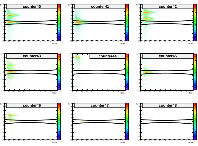
Figure 3.7 (a) The pion ∆T distribution in counter 40 of sector 3 shows two

peaks at 0.1 ns and 3.9ns (side band peaks), which are fit by

two Gaussian functions (red curves) to get the shift parameters.

(b) The same ∆T distribution with ∆T shift correction. . . 43

Figure 3.8 The pion ∆T versus pπ distribution with upper/lower ∆T cut

limits from counter 40 to 48 of sector 3. . . 43

Figure 3.9 The pion ∆T versus pπ distribution with upper/lower ∆T cut

limits from counter 40 to 48 of sector 3 after the ∆T shift

cor-rection. . . 44

Figure 3.10 (a) Proton ∆T distribution with Gaussian fit function (red

curve) at 0.4 GeV/c< pπ <0.6 GeV/c for sector 3. (b) Proton

∆T versus pproton distribution with upper/lower ∆T cut limits

for sector 3. . . 45

Figure 3.11 The proton ∆T versus pπ distribution with upper/lower ∆T

(15)

Figure 3.12 The proton ∆T versus pπ distribution with upper/lower ∆T

cut limits for counter 40 to 48 of sector 3 after the ∆T shift

correction. . . 47

Figure 3.13 The differences between generated and reconstructed protons

are presented by the black distributions for differentpp atθp =

15◦. The blue lines indicate the Gaussian fits. . . 48

Figure 3.14 The ratio between Gaussian fit peak positions (in Fig. 3.13) and

corresponding reconstructed momentum values, δp/p, plotted

against the reconstructed proton momentum (p) is presented

by the black circles, and the blue lines show the corresponding

fit functions. . . 49

Figure 3.15 Fit parameters of δp/p versus (p) distributions plotted against

the reconstructed protonθis presented by the black points, and

the blue lines show the corresponding fit functions. Here par[0],

par[1], and par[2] correspond to the fit parameters in Eq. (3.14). 50

Figure 3.16 The example missing mass squared distributions of the spec-tator without any kinematic corrections (black line), with only electron momentum corrections (blue line), and with both elec-tron momentum and proton energy loss corrections (red line) are plotted for sector 4, where the fit parameters in the statis-tics legend box correspond to the red-line Gaussian function

fit. . . 51

Figure 3.17 The µ2_mism_spector versus detector sectors without any kinematic

corrections (black squares), with only electron momentum cor-rections (red triangles), and with both electron momentum and

proton energy loss corrections (blue dots). . . 52

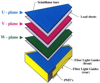
Figure 3.18 The U, V, and W coordinate distributions in the

electromag-netic calorimeter. The green area represents the selected events

after the cuts. . . 52

Figure 3.19 TheV coordinate distribution in the electromagnetic

calorime-ter. Red lines represent the hole cut limits. . . 53

Figure 3.20 θe versusφe distributions of electrons are plotted for six sectors

for experiment (left) and simulation (right) reconstructed data each side by side within the 0.8 GeV<|p~e|<1.0 GeV

momen-tum interval. The blue lines show the fiducial cut boundaries

(16)

Figure 3.21 Example φe distributions of electrons in sector 4 for data with

0.8 GeV< |~pe| <1.0 GeV before (blue) and after (green)

fidu-cial cuts. . . 55

Figure 3.22 θe versus p distributions of electrons in all six sectors are

com-pared for experiment (left) and simulation (right) reconstructed data simultaneously each side by side. The top and bottom

black lines show the θe cut boundaries, and the middle paired

black lines show removed regions, which are reflected in Fig. 3.20

by the low event-rate bands. . . 56

Figure 3.23 (a) Typical exampleφ distribution of pions from the 0.2 GeV<

|~pπ−| < 0.4 GeV and 28◦ < θ_π− < 30◦ intervals in sector 1, which are fit by the function (Eq. (3.18)) shown by the red

line, where the corresponding fit parametersP4,P5, andP6 are

heights of the corresponding plateau regions of the trapezoid

function and P0, P1, P2, and P3 are corresponding φ values of

the inflection points. (b) Example φ versus θ distribution for

pions in sector 1 within the same momentum interval.

Corre-sponding fit parametersP0 and P1 of eachθ bin are marked as

stars and fit by the function (Eq. (3.19)) shown by the back line. 57

Figure 3.24 Exampleφversusθdistributions of pions after event selection in

sector 1 for 0.2 GeV< pπ− <1.2 GeV within 0.2 GeV increasing steps, and the fiducial cuts (blue lines) are plotted here for

sector 1. . . 58

Figure 3.25 φversusθ distributions of pions in differentpπ− bins after event

selection are plotted for sector 1 for experiment (left) and sim-ulation (right) reconstructed data each side by side. The black

lines represent the fiducial-cut boundaries. . . 58

Figure 3.26 θ versus p distributions of pions in six sectors are compared

for experiment (left) and simulation (right) reconstructed data each side by side. The middle paired black lines show the re-moved regions, which are reflected in Fig. 3.25 by the verti-cal low event-rate bands, and the bottom black lines represent

θ > θπ−

(17)

Figure 3.27 (a) Typical example for a φ distribution of protons from the 0.2 GeV < |~pproton| < 0.4 GeV and 28◦ < θproton < 30◦

in-tervals in sector 1, which is fit by the function Eq. (3.18) and

plotted as the red line. The corresponding fit parameters P4,

P5, and P6 are heights of the corresponding plateau regions of

the trapezoid function, and P0, P1, P2, and P3 are the

corre-sponding φ values of the inflection points. (b) The φ versus θ

distribution of protons for sector 1 within the same momentum

interval. Corresponding fit parametersP0 and P1 of eachθ bin

are marked as stars, fit by the function Eq. (3.19), and shown

by the black lines. . . 60

Figure 3.28 Example φ versus θ distributions for protons in sector 1 for

0.2 GeV < pproton < 1.8 GeV within 0.2 GeV increasing steps

and the fiducial cuts (blue lines) for sector 1. . . 61

Figure 3.29 φ versus θ distributions of protons plotted for six sectors for

experimental experiment (left) and simulation (right) recon-structed data each side by side. The blue lines represent

fiducial-cut boundaries. . . 62

Figure 3.30 θversuspdistributions of protons in all six sectors are compared

for experimental (left) and simulation (right) reconstructed data each side by side. The middle paired black lines show the re-moved regions, which are reflected in Fig. 3.29 by the vertical

low event-rate bands. . . 63

Figure 3.31 TheM_s2 distribution with the two cut limits represented by the

red lines illustrates the exclusive event selection process. . . 64

Figure 3.32 (Color online) The|P~s|distribution of experimental data (black

line) and simulation (blue line) where “green” and “red” filled areas represent the integral of the blue distribution from 0 MeV

to 200 MeV and above 200 MeV, respectively. . . 65

Figure 3.33 (a)(Color online) The black line represents the missing

momen-tum distribution (|P~s|) of the unmeasured proton from

experi-mental data. Based on the CD-Bonn potential [28], the Monte Carlo simulated scaled proton momentum distribution leads to the red line and the detector-smeared simulated scaled distribu-tion to the blue line.(b) The zoomed plot of (a) to investigates

(18)

Figure 4.1 Flowchart showing the main steps of the detector and reaction

simulation process. γ∗n(p)→pπ−(p) events are generated by a

realistic event generator, passed through GSIM [1] and GPP [2],

and cooked by RECSIS [3]. . . 66

Figure 4.2 (a) W distributions of exclusive quasi-free events of

experi-mental data (black) and the corresponding simulated distribu-tion for the MAID98 (blue), MAID2000 (magenta), MAID2003

(green), and MAID2007 (red) versions. (b) Q2 _{distributions}

for the experimental events and the corresponding simulatied

events of (a). . . 68

Figure 4.3 Event start time (t0) distributions of the exclusive quasi-free

events for experimental data (left) and simulation with smear-ing factor f=0.9 (right) are fit by Gaussian functions (red curves). The corresponding fit parameters are listed in the statistic boxes,

respectively. . . 70

Figure 4.4 The σ of t0 versus f from the simulation events are fit by a

linear function (blue), and the red line corresponds to the theσ

oft0from the measured exclusive quasi-free events. Thef value

corresponding to the cross point is used to smear the simulated

detector SC resolution. . . 71

Figure 4.5 The fitted σ values of M_s2 distributions depending on different

a = b = c values are plotted as black points. These are fit

by a linear function (blue). The red horizontal line represents

the fitted σ values of M_s2 distributions from the experimental

reconstructed events. The value of a = b = c corresponding

to the cross point is used to smear the simulated detector DC

resolution. . . 72

Figure 4.6 The M2

s distributions of the exclusive quasi-free events for

ex-perimental data (left) and simulation with smearing factors

f = 0.9 and a = b = c = 2.5 (right) are fit by Gaussian

functions (red). The corresponding fit parameters are shown in

their statistics legend boxes. . . 72

Figure 5.1 W and Q2 _{binning for the} _π− _{electroproduction events, where}

vertical and horizontal lines are shown as the lower and upper

(19)

Figure 5.2 Example cosθ∗ and φ∗ binning for the π− electroproduction

events in 1.2 GeV < W < 1.225 GeV and 0.4 GeV2 < Q2 _<

0.6 GeV2 bin, where vertical and horizontal lines show the lower

and the upper bin limits. . . 75

Figure 5.3 Bin centering corrections RBC as a function of cosθ∗ and φ∗ in

the W = 1.2125 GeV and Q2 _{= 0}_._{5 GeV}2 _bin. _{. . . .} ₇₇

Figure 5.4 (a) Measured electron vertex (Ze) distributions for full target

events (black) and scaled empty target events (red). (b)The black distribution is kept the same as (a), and the vertex

distri-bution for scaled empty target events is shifted to (Ze−1.5 mm)

(red). . . 79

Figure 5.5 Ze distributions for full-LD2-target (black) and scaled

empty-target events (red) are plotted together in one canvas and

com-pared with these of the empty target subtracted fullLD2 target

events sector by sector. . . 79

Figure 5.6 Feynman diagrams of the radiative effects in theπ−

electropro-duction. (a) and (b) Brehmsstrahlung, (c) Vertex correction,

and (e) Vacuum polarization, as used by [48]. . . 81

Figure 5.7 M2

s distributions for measured (black) and simulatedγ∗n(p)→

pπ−(p) (blue), as well as simulated γ∗p → pπ−π+ events are

plotted with theM2

s cut limits. . . 82

Figure 5.8 M_s2distributions for measured (black) and simulatedγ∗n(p)→

pπ−(p) (red) events are plotted with theM2

s cut limits forW =

1.2125 GeV, Q2 _{= 0}_._{5 GeV, and cos}_θ∗ ₌ ₋₀_._{3 in} _φ∗

π− = 100◦,

140◦_{, 180}◦_{, 220}◦_{, 260}◦_{, and 300}◦ _{bins individually. . . .} ₈₃

Figure 5.9 W dependent normalized yield distributions in the eD → e0X

process are presented for data with black stars and for Os-ipenko’s world-data parameterization with magenta stars in

individual Q2 _{bins from 0}_._{4 GeV}2

to 1.7 GeV2 in steps of

∆Q2 = 0.1 GeV2. . . 85

Figure 6.1 The whole analysis process flowchart . . . 87

Figure 6.2 Exclusive (black points) and quasi-free (green squares) cross

sections in µb/sr are represented for W = 1.2125 GeV and

(20)

Q2 _{= 0}_._{7 GeV}2

. . . 90

Q2 _{= 0}_._{9 GeV}2_{. . . .} ₉₁

Q2 _{= 0}_._{5 GeV}2_{. . . .} ₉₂

Q2 _{= 0}_._{5 GeV}2

. . . 93

Figure 6.7 The ratios ofRF SI(Wi, Q2,cosθπ∗−, φ_π∗−) overRF SI(Wi, Q2,cosθπ∗−)

are represented by Blue points for different φ∗_π− at 1.2 GeV <

Wi < 1.225 GeV and 0.6 GeV2 < Q2 < 0.8 GeV2. The

in-dividual plot shows the ratios for different cosθ∗_π− bins. The

three lines from bottom to top correspond to 0.95, 1, and 1.05,

Figure 6.8 The ratios ofRF SI(Wi, Q2,cosθπ∗−, φ_π∗−) overR_{F SI}(W_i, Q2,cosθ_π∗−)

are represented by Blue points for different φ∗_π− at 1.2 GeV <

W < 1.225 GeV and 0.6 GeV2 < Q2 _<₀_._{8 GeV}2_{. The}

individ-ual plot shows the ratios for different cosθ∗_π− bins. The three

lines from bottom to top correspond to 0.95, 1, and 1.05, respectively. 95

Figure 6.9 RF SI versus θ∗π− distribution example for individual W bins,

which are increasing by 0.025 GeV in the range of 1.1 GeV <

W < 1.725 GeV for 0.4 GeV2 < Q2 _< ₀_._{6 GeV}2_{. The red}

and black points correspond to RF SI binned in Wi and Wf,

Figure 6.10 RF SI versus θπ∗− distributions example for individual W bins,

which are increasing by 0.025 GeV in the range of 1.1 GeV <

W < 1.725 GeV for 0.6 GeV2 < Q2 _< ₀_._{8 GeV}2_{. The red and}

black points correspond toRF SI binned in Wi and Wf, respectively. 97

Figure 6.11 RF SI versus θπ∗− distributions example for individual W bins,

which are increasing by 0.025 GeV in the range of 1.125 GeV<

W < 1.6 GeV for 0.8 GeV2 < Q2 < 1.0 GeV2. The red and

(21)

Figure 6.12 Example of the cosθ_π∗− dependent structure functionsσT +σL

(top row), σT T (middle row), and σT L (bottom row ) for W =

1.2125 GeV at Q2 _{= 0}_._{5 GeV}2

(left column), Q2 _{= 0}_._{7 GeV}2

(middle column), and Q2 _{= 0}_._{9 GeV}2 _{(right column) that are}

extracted for the exclusive (black points) and quasi-free (green squares) cross sections and compared with the predictions of the SAID (magenta points) and MAID2000 (blue points) mod-els. The solid black bars represent the corresponding systematic uncertainties. The Legendre polynomial expansions are fitted

to the corresponding structure function data for π− angular

momenta up tol = 2. . . 99

Figure 6.13 The ∆T distribution of pions in six sectors. The black, blue,

and red lines represent the 4σ, 3σ, and 2σ cut boundaries,

re-spectively. . . 103

Figure 6.14 The ∆T distribution of protons in six sectors. The black, blue,

and red lines represent the 4σ, 3σ, and 2σ cut boundaries,

Figure 6.15 (Color online) The φp versus θp distributions for six sectors

without proton fiducial cuts. The magenta, blue, and black lines represent loose, chosen, and tight proton fiducial cuts,

Figure 6.16 (Color online) The spectator missing mass squared M2

s

distri-butions for data (black curve) and simulation (blue curve). The black, red, and blue vertical lines represent loose, chosen, and

tightM2

s cuts, respectively. . . 105

Figure 6.17 (Color online) The spectator missing momentum |P~s|

distribu-tions for data (black curve) and simulation (blue curve). The black, red, and blue vertical lines represent loose, chosen, and

tight|P~s| cuts, respectively. . . 106

Figure 6.18 The normalized cumulative “spectator” proton momentum dis-tributions from different deuteron potentials. The black, blue, and red points represent the CD-Bonn, Paris, and Hulthen

(22)

Figure 6.19 The φ∗_π− dependence of the exclusive cross sections with and without radiative correction are marked as red points and black

squares, respectively for an example at W = 1.2125 GeV and

Q2 _{= 0}_._{7 GeV}2_{. The individual plots correspond to different}

cosθ_π∗− bins. . . 110

Figure 6.20 The ratios of W integrated inclusive cross sections of σOsipenko

overσY e marked as black stars are plotted againstQ2. The red

dot lines represent the Q2 _{averaged ratios. . . .} ₁₁₁

Figure 6.21 The ratios of Q2 _{integrated inclusive cross sections of} _σ

Osipenko

overσY e marked as black stars are plotted against W. The red

(23)

Chapter 1 Introduction and Overview

What’s the origin of more than 98% of the visible mass - that’s everything in the

universe, we sense and see around us? Visible matter is everything made of atoms,

which get their mass mainly from the atomic nucleus. The nuclei of atoms are

com-posed of nucleons, namely protons and neutrons. The proton and neutron, each made

of three valence quarks, are much more massive than the sum of their constituents.

Where does all this “extra” mass come from? In order to answer this question, we

have to understand how the quarks interact via the exchange of gluons, how quarks

bind together via strong interaction, and how gluons interact with each other. The

fundamental theory of the strong interaction is Quantum Chromodynamics (QCD),

which is very successful at predicting reactions with large momentum transfer, Q2,

within the perturbative regime with current quarks and gauge gluons as the

funda-mental degrees of freedom. However when Q2 _{drops down to the non-perturbative}

regime, there is a transition to completely different degrees of freedom, the dressed

quarks and gluons as well as the mesons and nucleons, which prevents us from having

a direct QCD description of the phenomena corresponding to hadronic physics, such

as the structure of the nucleon and its excitations (N∗).

The most fundamental approach to resolve this difficulty is to develop accurate

numerical simulations of QCD on to a four-dimensional Euclidean space-time lattice

(LQCD) [35], which is the only way to rigorously test QCD at present. LQCD makes

significant progress on calculating some basic properties of baryons, such as masses

(24)

challenging issues. Therefore, it is equally important to develop other complementary

nonperturbative methods based on the QCD approach to interpret the real world

properties, and the Dyson-Schwinger equations (DSEs) are such an approach. It is

based on infinite tower of coupled integral equations [60], which is discussed later.

Alternatively, hadron models with effective degrees of freedom have been constructed

to interpret data, such as constituent quark models [20], MIT-bag models [36], and

Nambu-Jona-Lasinio (NJL) models [41].

All these non-perturbative approaches need experimental data to test and

im-prove their predictions. Therefore we need to accumulate sufficient and precise data

on meson electroproduction reactions to pin down the distance-dependent structure

of the nucleon and its excitations, in order to push the development of quark models

and QCD-based calculations forward. Due to the short lifetimes of N s∗, it is

im-possible to observe these excitation states directly. In the experiment, we can study

N s∗ via products of their decays. There are a couple ways to study N s∗ production,

i.e., electroproduction and photoproduction of pseudo-scalar or vector mesons. The

electromagnetic vertex of the meson electroproduction is well described by Quantum

Electrodynamics (QED), while the hadron scattering governed by the strong

inter-action is the only unknown part in the electroproduction process. Furthermore, the

virtual photon exchange of the electroproduciton allows us to study hadronic

proper-ties at differentQ2_{regimes, which is crucial in understanding of the internal dynamics}

of the strong interaction in the non-perturbative regime. In reactions of meson

elec-troproduction off nucleons, we are interested in the resonance processes, in which a

virtual photon excites the nucleon to its excitated state (N∗), with then decays to

one meson or more and nucleon. Beside this, the non-resonance processes in this

reaction are treated as background in the reaction models to extract the resonance

information.

(25)

elec-troproduction off the proton in the hydrogen target. Hence flavor-dependent analyses

of excited light-quark baryons are lacking experimental data off the neutron, which is

due to the fact that there is no free neutron target. Deuterium becomes to be one of

the best alternate targets for neutrons, whose nucleus consists of one proton and one

neutron, because it is the simplest and most loosely bound system of neutron.

How-ever, due to the neutron being bound in the deuteron, a few effects must be studied

in order to extract the neutron information, such as, Fermi motion, off-shell effects,

and final state interactions (FSI). The goal of this work is to provide the exclusive

and quasi-freeγ∗n(p)→pπ−(p) reaction cross sections from deuterium target, as well

as kinematical FSI contribution factor RF SI that can be determined from the data

itself. This thesis work concentrates on the study of the bound neutron resonance

via meson electroproduction, which will improve our knowledge of the Q2 _evolution

of the resonance states off the bound nucleon system and aid our understanding of

the structure and interaction of hadrons.

1.1 QCD and Non-Perturbative Approaches

QCD

QCD describes the interaction between quarks and gluons, which we believe are the

fundamental degrees of freedom that make up hadronic matter. Quarks are one type

of fundamental particles, it means that they are not composed of any other particles.

There are six known, electrically-charged, different-flavored quarks, which are listed

in the Tab. 1.1. Each quark has its own antiquark.

Quarks interact with each other only through intermediate agents “gluons”, which

are the exchange particles that couple to the color charge in QCD. This is analogous

to the electromagnetic interaction in which photons are exchanged between

(26)

Table 1.1: Summary of quark properties.

Name Symbol Charge Isospin (I3) Mass (MeV/c2)

Up u +2/3 +1/2 2.3±1.2

Down d −1/3 −1/2 4.8±0.8

Charm c +2/3 0 1275±25

Strange s −1/3 0 95±5

Top t +2/3 0 173210±510

Bottom b −1/3 0 4180±30

gluons simultaneously carry color and anticolor charge. Since gluons are vectors in

the adjoint representation of color gauge group SU(3), there are eight gluons. By

their exchange the eight gluons mediate the interaction between particles carrying

color charge, i.e., not only the quarks but also the gluons themselves. This is an

important difference to QED, where the electromagnetic field quanta have no charge,

and therefore cannot couple at lowest order with each other. The elementary

pro-cesses of QCD include emission and absorption of gluons (Fig. 1.1(a)); production

and annihilation of quark-antiquark pairs (Fig. 1.1(b)); and coupling three or four

gluons to each other (Fig. 1.1(c) and (d)). QCD is a non-abelian gauge theory whose

Figure 1.1: The fundamental interaction diagrams of QCD [56]: (a) emission of a gluon by a quark, (b) splitting of a gluon into a quark-antiquark pair, (c) and (d) self-coupling of gluons.

dynamics are governed by the Lagrangian [52], which is represented by

LQCD =

X

q

¯

ψq,a(iγµ∂µδab−mqδab)ψq,b−

X

q

¯

ψq,agsγµtCabA C µψq,b−

1

4F

A µνF

Aµν

(27)

where γµ _{are the Dirac} _γ _{matrices. The} _ψ

q,a are quark-field spinors for a quark of

flavor q and mass mq, with a color-index a (a = 1 to 3, quarks have three “colors”).

AC

µ correspond to the gluon fields, with C running from 1 to 8 (there are 8 kinds of

gluons). Furthermore,tC

ab (tCab ≡λCab/2) are eight 3×3 matrices that are the generators

of the SU(3) group. The field tensor FA

µν is given by

F_µνA =∂µAAν −∂νAAµ −gsfABCABµA C

ν, (1.2)

where the fABC are the structure constants of the SU(3) group, and gs is the QCD

coupling constant calculated by

αs(Q) =g2s/4π, (1.3)

αs(Q) =

2π β0ln(Q/ΛQCD)

, (1.4)

β0 = 11− 2

3nf, (1.5)

wherenf is the number of quark flavors that are involved in the process, and ΛQCD is

the fundamental cut-off parameter of QCD, whose value is experimentally determined

as ΛQCD ∼200 MeV/c [56].

The first term in the Eq.(1.1) represents the part of the free quark fields, the second

term corresponds to the quark-gluon interactions (Fig. 1.1(a) and (b)). The quark

interacts with gluons is in a way similar to the electrons interacting with photons in

QED. Gluons are physical degrees of freedom and therefore must carry energy and

momentum themselves. Thus the third term in the Lagrangian is needed to describe

gluon self-interactions. Since gluons carry color charges, their self-interactions are

responsible for many of the unique and important features of QCD, such as asymptotic

freedom, color confinement, and chiral symmetry breaking [50].

The second term in Eq. (1.5), −2

3nf, comes from quark-antiquark pair screening.

(28)

gluon-gluon vertices (Fig. 1.1). Thus the gluons self-coupling causes a color

anti-screening effect.

Three important characteristic QCD features are listed as following

• Asymptotic freedom: From Eq. (1.4), this Q-dependence of the coupling strength

corresponds to the dependence on separation. For very high Q values (very

small distance), the interquark coupling decreases, vanishing asymptotically. In

the limit Q→ ∞, quarks can be considered as “free”, this is called asymptotic

freedom.

• Confinement: In the very low energy domain (very large distance), the interquark

coupling increases so strongly that it is impossible to detach individual quarks

from hadrons (confinement) [56]. Although the confinement hypothesis has not

been directly derived from QCD.

• Dynamical chiral symmetry breaking: Contrary to confinement, we are able to

understand it better even though it is an other typical low-energy feature of

QCD. Since in the low-energy domain of QCD, the proton is composed of three

valence quarks: two up quarks with mu ∼ 2.3 MeV and one down quark with

md∼4.8 MeV, only contributing about 9.4 MeV to the rest mass of the proton

( 938 MeV). It turns out that chiral symmetry is realized in this regime. The

source of the bulk of the proton’s mass is QDC binding energy, which arises

from QDC dynamical chiral symmetry breaking [57], and an effective quark

mass is generated [36].

Lattice QCD (LQCD)

LQCD is QCD solved on a discrete four dimensional Euclidean space-time lattice

with spacing a, with quark fields placed on sites and gauge fields on links between

(29)

quan-tum field theory finite [52]. When a→0, the continuum theory is recovered. LQCD

is defined by allowing the numerical evaluation of the path integral, which is based

on a non-perturbation calculation. Progress in LQCD has required a combination

of improvements in formulation, numerical techniques, and in computer technology,

allowing these simulations to calculate correlation. The practical calculation results

of LQCD come with both statistical and systematic errors due to the limitation of

the efficiency of algorithms and the availability of computational resources. The

sta-tistical errors correspond to the use of Monte-Carlo integration, the systematic errors

come from using non-zero values of a. Since LQCD is a regularization of QCD, the

only tunable input parameters for lattice calculation are the strong coupling constant

αs and the quark masses for each flavor, which are determined using experimental

inputs. In this way, if QCD is the correct theory of strong interactions, all predictions

of LQCD have to agree with experimental data, and the nucleon and pion structure

from lattice QCD simulations by using a physical pion mass is achieved [13].

Dyson-Schwinger Equations (DSE)

The DSEs are coupled infinitely tower integral equations, which are a general

rela-tionship between Green’s functions in quantum field theories (QFT) [60]. Solving

these equations provides a solution of QDC. The DSEs include the Bethe-Salpeter

equation (BSE) which is a tool to calculate the properties of relativistic two-body

scattering and bound states. For studies based on DSEs, it is unavoidable to deal

with the infinite tower of coupled integral equations. For practical purposes, the

cur-rent approach of DSEs truncates the tower at some point. This means that the tower

of integral equations must be limited to some n, where n is the maximum number

of legs on any Green’s function included in the self-consistent solution of the

equa-tions [60]. An Ansatz can then be introduced for the omitted terms. There is hope

(30)

of these truncated functions. One approach of studying the non-preturbative

prop-erties of hadrons is the combination of DSEs and Bethe-Salpeter equations (BSE).

There are some calculations related to this approach, which were performed upon

truncating the (anti)quark-quark interaction to a single gluon exchange, so-called

Rainbow-Ladder truncation [62]. Based on that, the details of recent studies on

me-son spectra have been published in Refs. [31] [32] [38]. Baryons have been studied

in the quark-diquark approximation [63]. Current interest of DSEs and BSE

combi-nation approach is the inclusion of interaction mechanisms beyond the leading term

[62], and in the extension to glueball [61] and tetraquark bound-states [37].

1.2 Single-Pion Electroproduction off the Moving Neutron

Single-pion electroproduction has been the main process in the study of the N −

N∗ transition form factors of the lower mass nucleon resonances such as P33(1232),

P111440, D13(1520),S11(1535), S11(1650), F15(1680), and D33(1700).

Data Status

The low-lying excited states of the proton have been studied in greater detail [19],

there is still very little data available on neutron excitations. Because of the inherent

difficulty in obtaining a free neutron target, a deuterium target is the best alternative.

From the SAID database [4], theπ− electroproductions off neutrons in the deuterium

are listed in the Tab. 1.2, in which, the ratioRπ−_/π+ was directly measured for most

available data. Even though the differential cross sections were measured directly,

they are only available for single or couple Q2 _{values and in parts of the whole}

resonance range. We need to accumulate sufficient and precise data for the neutron,

not only to study the isospin dependent structure of the nucleon and its excitations,

(31)

Table 1.2: Summary of the single pion electronproduction off bound neutron in the deuterium target withRπ−_/π+ = dσ(γν+n→π

−₊_p₎

dσ(γν+p→π++n) =

Rate(e+d→e+π−+p(p))

Rate(e+d→e+π+₊_n₍_n₎₎.

Reaction Observable W value Q2 _value _{Lab/experiment}

GeV GeV2

en(p)→e0π−p(p) Rπ−_/π+ 2.15, 3.11 1.2, 4.0 Cornell/WSL [17]

ep(n)→e0π+n(n)

en(p)→e0π−p(p) dσ/dΩπ 2.15, 2.65 1.2, 2.0 Cornell/WSL [18]

ep(n)→e0π+n(n)

en(p)→e0π−p(p) Rπ−_/π+ 1.28-1.71 0.5 NINA [64]

ep(n)→e0π+n(n)

en(p)→e0π−p(p) Rπ−_/π+ 1.3-1.7 1.0 NINA [49]

ep(n)→e0π+n(n)

ep(n)→e0π+n(n) Rπ+_/π− 1.16, 1.232 0.0856, 0.0656 ALS [34]

en(p)→e0π−p(p)

en(p)→e0pπ−(p) σL, σT 1.15, 1.6 0.4 JLab-HallA [33]

en(p)→e0pπ−(p) σL, σT 1.95, 2.45 0.6, 1.0, 1.6, 2.45 JLab-HallC [39]

The six simplest pion electroproduction reactions off the free proton, bound

pro-ton, and bound neutron targets are summarized as

γ∗+p→π0+p, (1.6)

γ∗+p→π++n, (1.7)

γ∗+D(p)→π++n+ns, (1.8)

γ∗+D(p)→π0+p+ns, (1.9)

γ∗+D(n)→π−+p+ps, and (1.10)

γ∗+D(n)→π0+n+ps. (1.11)

All the listed single-pion reactions under the same experimental conditions are

in-cluded in the “e1e” run, which took data with the CLAS detector at JLab from

December 14th, 2002 to January 24th, 2003. The combined analysis of processes

Eq. (1.6)- (1.10) will provide the best possible experimental information about the

final state interactions and the off shell effects of the bound nucleon, which are

(32)

analyzed, which includes both resonance and non-resonance process, to extract

cor-responding cross sections off the neutron in the deuterium target in the resonance

region. The resonance process of interest Eq. (1.10) is shown in Fig. 1.2, where the

electron emits a virtual photon (γ∗) exciting the neutron to one of its excitations

(N∗), then the resonance decays to a π− and a proton (p). The initial proton in the

deuteron is treated as a spectator (Ps), which will be discussed in Chapter 3 that

discusses how to isolate the quasi-free process.

Figure 1.2: The resonance process of single-pion electroproduction off a neutron in deuterium. The initial proton in the deuteron is treated as the spectator, named as

Ps.

Kinematic

Before we introduce the kinematics of the scattering from a bound neutron in a

deuteron, we first consider the case of scattering from a free neutron that is at rest

in the lab frame, then the chosen variables Wi and Q2 are defined as:

W_irest =q(qµ₊_nµ₎2 ₌q₍_pµ_{+ (}_π−₎µ₎2 ₌_Wrest

f , (1.12)

(Qrest)2 =−(qµ)2 = (eµ−eµ0)2 , (1.13)

whereqµ _{presents the four momentum of the virtual photon.} _Wrest

i and (Qrest)2

(33)

transfer of the virtual photon for this scattering respectively, which are determined

in the leptonic interaction plane that is shown in Fig. 1.6 with the gray color. In

addition, we also need to determine two body final state pµ _{and (}_π−₎µ_{. In general,}

two final particles need to be described by 4×2 = 8 components of their four vector

momentum. Indeed, with the knowledge that they are all on mass shell, it gives

two restrictions (E_j2 −k2_j = m2_j;j = 1,2). Furthermore, the energy momentum

conservation laws impose four additional constraints for four momentum components

of the final particles. So we only need two kinematics variables to determine the

hadronic two body final state. Eventually, we end up with four variables to represent

the γ∗n(p)→pπ−(p) cross section.

For the kinematics of the process Eq. (1.10) that is the scattering from a bound

neutron in a deuteron, we have to consider the influence on the final cross sections of

Fermi motion, off-shell effects, and the final state interaction, which are introduced

next.

The Fermi Motion

In the process Eq. (1.10), where the initial neutron is moving around “quasi-freely”

in the deuteron in the lab frame. By measuring all final particles e0, p, and π−

exclusively, energy and momentum conservation imply that the sums of the

four-momenta before and after the reaction are identical:

qµ+Dµ= (π−)µ+pµ+pµ_s ,

qµ+pµ_i +nµ= (π−)µ+pµ+pµ_s ,

(1.14)

where Dµ is the four-momentum of deuteron that is at rest in the lab frame, Dµ =

(0, mD). nµand pµi correspond to the four-momentum of the neutron and the proton,

respectively, that are moving and loosely bound in the deuteron in that frame. The

outgoing missing protonpµ

(34)

Eq. (1.14) by

pµ_s =qµ+Dµ−(π−)µ−pµ, (1.15)

and the momentum of this proton is calculated by

~

Ps =~q−π~−−~p. (1.16)

Ignoring the off-shell effects at this moment, we focus on the motion first. In the

quasi-free process of the reaction Eq. (1.10), where the initial proton is treated as a

“spectator” that is totally unaffected by the interaction, thus pµ_i = pµ

s in Eq. (1.14)

(ignoring the off-shell effects). Then we can rewrite the Eq. (1.14) by

qµ+nµ= (π−)µ+pµ, (1.17)

and the initial neutron momentum is reconstructed by

~n=π~−₊_~_p₋_~_q. _(1.18)

For the quasi-free process, by comparing Eq. 1.16 with Eq. 1.18, we get

~

Ps=p~i =−~n. (1.19)

In contrast to the free neutron case, the neutron is now moving around with the

Fermi momentum, which is reconstructed from Eq. (1.18) and graphed in Fig. 1.3.

This motion causes changes in the kinematics compared to scattering off a neutron

at rest in the lab frame. Thus, in order to define the proper electron scattering

plane, we first boost eµ, (e0)µ, pµ, and (π−)µ from the lab frame into the neutron

rest frame with the boost vector calculated from nµ (Eq. (1.17)). In this frame, the

variablesW_i,W_f andQ2 _{are calculated from Eq. (1.12) and Eq. (1.13), as well as the}

electron scattering plane is defined. Then Wf and Q2 are selected to represent the

scattering cross sections off the moving neutron in the deuteron. So for this work,

the final reported cross sections are not influenced by the Fermi momentum of the

(35)

(GeV) n

0 0.5 1 1.5 2

Events

0 2000 4000 6000 8000 10000 12000

n Exclusive

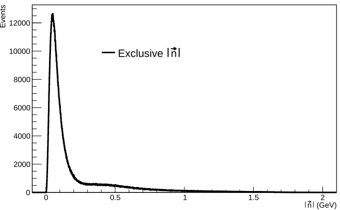
Figure 1.3: The momentum distribution of initial neutron in the exclusiveγ∗n(p)→

pπ−(p) process, which is moving in the deuteron in the lab frame.

Off-shell Effects

As mentioned previously, the bound neutron is also off-shell beside moving around

in the deuteron. Even in the quasi-free process (isolating the quasi-free process is

discussed in the Chapter 3), pµ_i is not equal to pµ_s due to the fact that the initial

proton pi is off-shell and outgoing “spectator” proton ps is on-shell in the reaction

Eq. (1.10). However the relationp~i =p~s=−~n is not influence by the off-shell effects

in the quasi-free process. So we can reconstruct the off-shell neutron four momentum

bynµ_{= (}₋_P~

s, Mn) andEn =

q

(−P~s)2+ (Mn)2. So it is better to choose Wf, which

is well defined and measured directly from p and π−, rather than Wi, to present

the final cross section. In the “spectator” situation, in order to conserve energy and

momentum in the scattering process, we have set

Mn=mn−2

k2

n

2mn

−2MeV, (1.20)

reestablishing Wi = Wf. This can be seen in Fig. 1.4, where Wf is calculated by

(36)

which are presented by the black and red lines separately, and their peaks match

each other. For other possibleMnsettings, we get shifted or smearedWidistributions

(radiative corrected) compared to Wf. The boost vector (from the lab frame to the

CM frame) is calculated using the different Wi and Wf, then the influence of those

different boosts on the final cross section can be quantified. The result shows that

these effects on the final cross sections are marginal and are accounted for as a source

of systematic uncertainties described in Chapter 4.

W [GeV]

1.1 1.2 1.3 1.4 1.5 1.6

Yield

0 1000 2000 3000 4000 5000

f

W

move

n =mn

n

E

W

rest

n =mn

n

E

W

move

n

=mn-2K-2MeV

n

E

W

move

n

=mn+2K+2MeV

n

E

W

move

n

=mn+K+1MeV

n

E

W

move

n

=mn-K-1MeV

n

E

W

Figure 1.4: (Color online) The comparison ofW distributions. Black line presentsWf,

blue line shows Wi calculated by setting nµ = (−P~s, En) (En with Eq. (1.20)). The

other colors present the Wi distribution by setting nµ to (−P~s, mn) (cyan), (0, mn)

(magenta), (−P~s, mn+ 2 k2

n

2mn+ 2MeV) (blue), (−

~

Ps, mn+ k2

n

2mn + 1MeV) (orange), and

(−P~s, mn− k

2

n

2mn −1MeV) (green).

The Final State Interaction (FSI)

In the reaction process Eq. (1.10), which is shown in Fig. 1.5 (a), with a|P~s|<200 MeV

(37)

the resonance process, it is possible to have final state interactions, such as pp

re-scattering and pπ re-scattering shown in Fig. 1.5 (b) and (c) respectively. It

corre-sponds to the situation in which the outgoing proton orπ−interacts with the spectator

proton (Ps). Thus, the four momentum of the final state particles are changed due to

these final state interactions. After isolating the quasi-free process, the kinematical

FSI contribution factor RF SI will be extracted from the data itself, and the details

will be discussed in the Chapter 6. It is also possible to have other kinds of FSI,

i.e. in the process Eq. (1.9) or (1.10), it is possible to have π0 +ns → π−+p and

π−+ps → π0 +n final state interactions in these processes, which can increase or

decrease the final stateπ− andpproduction. If we want to quantify the contribution

of this kind of FSI from the data itself, a combined analysis of pion electroproduction

off the free proton, the bound proton, and the bound neutron in the “e1e” run is

needed. In this thesis, this kind of final state interactions are not quantified from the

data itself.

d

n

ps

p

g* _p_

d

n

ps

p _p

1

p2

p_

d

g*

(a)

(b)

(c) n

p

ps

g*

p' p

-p'

-Figure 1.5: Kinematic sketch as in the text for the three leading terms in γ∗+D→

π−+p +p process (a) quasi-free, (b) pp re-scattering, and (c) pπ− re-scattering.

(38)

Boosting of the Kinematic Variables

p

-p



z



x



y

e



p*

*

p



n

*

p







_,

q

' ' '

_,

_k

_,

_E

e



E

k

e



,

Figure 1.6: Kinematics of π− electroproducton off a moving neutron. The leptonic

neutron rest frame plane is formed by eµ _and _eµ0_{, where} _k_, _E_, _k0_{, and} _E0 _are

corre-sponding momentum and energy of the incoming and outgoing electrons. qµ is the

virtual photon four momentum and ν is the transfered energy. The hadronic CM

frame plane is determined by final particles p and π, here θ∗_p and θ∗_π are their polar

angles and φ∗_π the azimuthal angle ofπ−.

In order to get the correct variables to present the final cross sections of π−

elec-troproduction off the neutron in the deuterium target, we boost first all particles’ four

momenta from the lab frame (deuterium at rest) into the neutron at rest frame with

the boost vector β~1 =−~n/En, where ~n and En are calculated from nµ (Eq. (1.17)).

Then the invariant mass Wf and the momentum transfer Q2 are calculated by the

Eq. (1.12) and (1.13) in this frame. In addition, by setting the coordinates in this

frame, ˆznrest parallel to the virtual photon direction and ˆynrest perpendicular to the

electron scattering plane, we ensure that ˆxnrest is staying in the electron scattering

plane and is set to be ˆx direction in the final coordinate system. Secondly, we

di-rectly boost all particles’ four momenta from the lab frame into the CM frame with

the boost vectorβ~2 =−(p~+π~−)/(Ep+Eπ−), then set the ˆz_CM parallel to the virtual

(39)

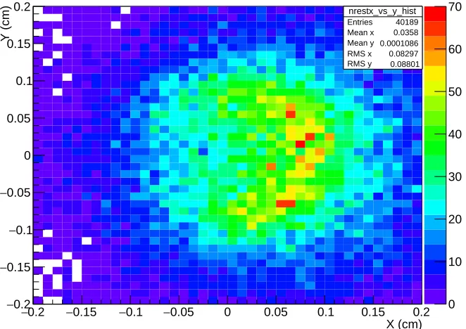
effects, it is better to set the final ˆz parallel to ˆzCM. The X and Y projections of

the ˆznrest in the CM frame are plotted against each other for final-state-interaction

dominated events and quasi-free events, which are shown in Fig. 1.8 and 1.7,

respec-tively. It turns out that the spread of these distributions around zero correspond to

the angle difference between ˆznrest and ˆzCM, which are 5.4◦ for final-state-interaction

dominated events in the exclusive process and < 1◦ for quasi-free events. Although

the final-state-interaction dominated events show significant spread, this coordinate

choice is the best way to present the quasi-free results for the bound neutron data.

The cosθ∗_π− and φ∗_π− are calculated ultimately in the CM frame. In summary, the

coordinates are set by:

ˆ

z = q~ ∗

|_q~∗_|, CM frame

ˆ

xis in the~k, ~k0 plane of the n rest frame and perpendicular to ˆz,and,

ˆ

y= ˆz×x,ˆ

(1.21)

which are shown in Fig. 1.6.

X (cm) 0.1

− −0.08 −0.06 −0.04 −0.02 0 0.02 0.04 0.06 0.08 0.1

Y (cm)

0.1 − 0.08 −

0.06 −

0.04 −

0.02 −

0 0.02 0.04 0.06 0.08 0.1

nrestx_vs_y_hist Entries 20281 Mean x 0.004428 Mean y −0.0001721 RMS x 0.0205 RMS y 0.02071

0 50 100 150 200 250 300 nrestx_vs_y_hist

Entries 20281 Mean x 0.004428 Mean y −0.0001721 RMS x 0.0205 RMS y 0.02071

Figure 1.7: TheX andY projections of the ˆznrestin the CM frame are plotted against

(40)

X (cm) 0.2

− −0.15 −0.1 −0.05 0 0.05 0.1 0.15 0.2

Y (cm)

0.2

−

0.15

−

0.1

−

0.05

−

0 0.05 0.1 0.15

0.2 _{nrestx_vs_y_hist}

Entries 40189 Mean x 0.0358 Mean y 0.0001086 RMS x 0.08297 RMS y 0.08801

0 10 20 30 40 50 60 70

nrestx_vs_y_hist

Entries 40189 Mean x 0.0358 Mean y 0.0001086 RMS x 0.08297 RMS y 0.08801

Figure 1.8: TheX andY projections of the ˆznrestin the CM frame are plotted against

each other for final-state-interaction dominated events.

Formalism

The cross section for the exclusive γ∗n → pπ− reaction with unpolarized electron

beam and unpolarized free neutron target is given by

d5_σ

dE0dΩ∗_π−dΩ_e0

= Γυ

E0,Ω_e0

dσ dΩ∗_π−

. (1.22)

Where the virtual photon flux that depends on the matrix elements of the leptonic

interaction is calculated by

Γυ

E0,Ω_e0

= α

2π2

E0 E

Kγ

(1−)Q2. (1.23)

Here α = 1/137 represents the electromagnetic coupling constant, corresponds to

the transverse polarization of the virtual photon,

= 1 + 2 |~q|

2

Q2

!

tan2θe

2

!−1

, (1.24)

and the photon equivalent energy is calculated by

Kγ =

W2−M_n2

2Mn

Measuring Strategic Communications

University of South Carolina

Scholar Commons

Exclusive π− Electroproduction off the Neutron in

Deuterium in the Resonance Region

Ye Tian

Dedication

Acknowledgments

Abstract

Table of Contents

List of Tables

List of Figures

Chapter 1

Introduction and Overview

QCD

Lattice QCD (LQCD)

Dyson-Schwinger Equations (DSE)

Data Status

Kinematic

The Fermi Motion

Off-shell Effects

The Final State Interaction (FSI)

d

d

d

Boosting of the Kinematic Variables

p

-p

z

x



y







n





,

q

,

k

,

E

e

E

k

e

,

,

Formalism

_,

_,

_k

_,

_E