Article
Diamagnetism of bulk graphite revised
Bogdan Semenenko and Pablo D. Esquinazi * 0000-0003-0649-1472
Division of Superconductivity and Magnetism, Felix-Bloch-Institute for Solid State Physics, Faculty of Physics and Earth Sciences, University of Leipzig, Linnéstraße 5, 04103 Leipzig, Germany;
[email protected] (B.S.)
* Correspondence: [email protected]; Tel.: +49-341-97-32-751
Abstract:Recently published structural analysis and galvanomagnetic studies of a large number of 1
different bulk and mesoscopic graphite samples of high quality and purity reveal that the common 2
picture assuming graphite samples as a semimetal with a homogeneous carrier density of conduction 3
electrons is misleading. These new studies indicate that the main electrical conduction path occurs 4
within 2D interfaces embedded in semiconducting Bernal and/or rhombohedral stacking regions. 5
This new knowledge incites us to revise experimentally and theoretically the diamagnetism of 6
graphite samples. We found that thec-axis susceptibility of highly pure oriented graphite samples is 7
not really constant but can vary several tens of percent for bulk samples with thicknesst&30µm, 8
whereas by a much larger factor for samples with smaller thickness. The observed decrease of 9
the susceptibility with sample thickness resembles qualitatively the one reported for the electrical 10
conductivity and indicates that the main part of thec−axis diamagnetic signal is not intrinsic of the 11
ideal graphite structure but it is due to the highly conducting 2D interfaces. The interpretation of 12
the main diamagnetic signal of graphite agrees with the reported description of its galvanomagnetic 13
properties and provides a hint to understand some magnetic peculiarities of thin graphite samples. 14
Keywords:graphite; diamagnetism; thickness dependence; susceptibility; interfaces; conductivity; 15
graphene 16
1. Introduction 17
Thec−axis diamagnetic susceptibility of graphite is very large and anisotropic [1–3]. According 18
to the literature of the last 50 years there is consent to interpret this large diamagnetism as due to 19
the Landau diamagnetic contribution of a certain density of free conduction electrons within the 20
graphene planes of graphite. The relatively low density of conduction electrons in graphite arises 21
from the overlap of the 2pzelectronic orbitals, normal to the graphene planes. Whereas the overlap 22
between those orbitals from the carbon atoms at neighbouring graphene layers, in both Bernal and 23
rhombohedral stacking orders, remains very weak, i.e. Van der Waals coupling, as the huge anisotropy 24
of the resistivity and magnetization indicates. 25
The calculations of the conduction-electrons magnetic susceptibility have been done in the 26
past taking into account an electronic band structure inferred from electric transport and magnetic 27
measurements [4–6]. In particular using the quantum oscillations in the electrical resistance, Hall effect 28
and magnetization, the Shubnikov-de Haas (SdH) and de Haas-van Alphen effects. All theoretical 29
models as well as the interpretation of the measured diamagnetism of graphite in those publications 30
assumed that high quality and pure graphite samples are homogeneous, structurally as well as 31
electronically. All free parameters of the band structure models were obtained from a comparison with 32
experimental data of different graphite samples [7]. Nowadays one may doubt about the accuracy of 33
the used models in particular because no electron-electron or spin-orbit coupling interactions were 34
included explicitly, plus the difficulties those calculations have to model the Van der Waals interaction 35
between the graphene layers. 36
The main problem those models and interpretation have, however, is directly related to the 37
misleading assumption that the experimental magnetic and electrical data correspond to homogeneous 38
bulk graphite samples. First experimental hints at odd with this assumption were obtained from the 39
magnetic field dependence of the Hall coefficient of kish graphite samples of different thickness [8,9]. 40
Namely, the amplitude of the SdH oscillations decreases the smaller the thickness of the samples. 41
For example, for a sample with thickness of 18 nm (which corresponds to a stacking of more than 42
50 graphene layers) one can barely recognize the field oscillations in the Hall coefficient, in clear 43
contrast to thicker flakes; for a review and discussion on these and other experimental results on 44
this issue see [10]. Moreover, a nonlinear increase of the resistance of graphite samples the smaller 45
their thickness was reported [11], which can be described as an anomalous increase in the estimated 46
absolute resistivity [12] the thinner the sample. Surprisingly, none of those studies [8,9,11] tried to 47
correlate the obtained results with the internal structure of the samples. 48
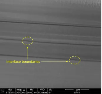
Figure 1.STEM picture of a comercial HOPG ( SPI) graphite lamella (∼400 nm thick) cut from a bulk sample measured also in this work. The electron beam is applied parallel to the graphene layers and normal to the mainc−axis of the graphite structure. The different grey colours indicate crystalline regions with different stacking order (Bernal or rhombohedral) or regions twisted around thec−axis by a certain angle respect to the neighbouring regions. Well defined two-dimensional interfaces are located between regions with different grey colors at the middle of the picture, which includes also interface boundaries (yellow ellipsoids). More STEM pictures (also with much higher resolution) obtained from different commercial HOPG samples and natural graphite can be seen in [10].
Experimental evidence obtained in graphite bulk samples and thin flakes the last 10 years reveals 49
that the observed thickness dependence of the magneto-electric properties of graphite has its origin 50
microscopy (STEM) studies, as example see Figure1, reveal the existence of two-dimensional (2D) 52
interfaces between regions with different stacking order and/or between regions with similar stacking 53
order but twisted around a commonc−axis [10]. The presence of two stacking orders, identified as the 54
majority phase called Bernal (ABABA...) and the rhombohedral (ABCABCA...) stacking order, has 55
been measured by high resolution x-rays diffraction (XRD) [15] of different samples including natural 56
graphite crystals, highly oriented pyrolytic graphite (HOPG) or kish graphite [10,16], in agreement 57
with previous reports [7,17]. It is important to note that these two stacking orders are not semimetals, 58
but semiconductors with energy gaps of 38±8 meV (Bernal) and 110±20 meV (rhombohedral), 59
obtained from the fits to the temperature dependence of the resistance between 2 K to 1100 K of a large 60
number of different samples of different origins [13]. 61
The galvanomagnetic results obtained for samples of different thickness indicate that a highly 62
conducting path in graphite samples is localized at the 2D interfaces [12–14,18], which upon twist 63
angle [10] or stacking order [19,20] they can even show superconducting properties [15,21–23]. The 64
origin of the SdH oscillations in the electrical resistance is related to the 2D interfaces, as recent detailed 65
electrical measurements clearly revealed [14]. All these recent results motivated us to study more 66
carefully the magnetization of graphite samples with smaller thickness than the usually reported 67
samples in the literature. Since the two stacking order phases are semiconducting, it is clear that 68
the diamagnetic signal of graphite cannot be intrinsic of the graphite structure, otherwise we would 69
have large changes of thec−axis susceptibility with temperature, which is not the case [7]. If the 70
large diamagnetic moment measured in large bulk samples of graphite is mainly due to the highly 71
conducting interfaces, taking into account STEM studies (see section 2) we expect then to observe a 72
non systematic variation of the diamagnetic response in bulk samples, even if the samples have similar 73
volumen and cut from the same sample. Also we would expect to see a decrease in the absolute value 74
of the diamagnetic susceptibility the smaller the interface number, i.e. the smaller the sample thickness. 75
In clear contrast to the technical requirements needed to study the electrical resistance of graphite 76
samples with thickness down to a single graphene layer, the measurement of the diamagnetic moment 77
of thin graphite samples with a commercial SQUID magnetometer is difficult or even impracticable. 78
For example, assuming one wants to measure the diamagneticc−axis magnetic moment of a graphite 79
flake of thickness×width×length equal to 1µm×0.2 mm×0.2 mm with an expected diamagnetic 80
c−axis susceptibilityχ∼ −2×10⁻⁵emu/g Oe, the expected diamagnetic moment at a field of 104Oe 81
applied parallel to thec−axis would bem . −2×10⁻⁸ emu, a value of the order of the error of 82
commercial SQUIDs nowadays. The expected small magnetic moment added to a not-easy handling 83
of such small thin flakes for that kind of measurements (without large backgrounds from substrates, 84
etc.) put already hard restrictions to perform such magnetization measurements. 85
In this work and besides the SQUID we have used a torque magnetometer that allowed us to 86
measure with high resolution the susceptibility of well ordered graphite flakes with thickness to 87
∼ 1µm and larger. The obtained results of the magnetic moment of highly oriented samples of 88
different sources and with both magnetometers show that the absolute value of the diamagnetic 89
susceptibility decreases the smaller the sample thickness. Our results can be considered as a first 90
experimental hint that agrees qualitatively with the thickness dependence of the conductivity of similar 91
samples. Our results suggest that the largest contribution to the diamagnetic susceptibility measured 92
in bulk samples is not intrinsic of the ideal graphite structure. 93
The manuscript is organized as follows: In the next section we discuss the density of interfaces 94
following the information of a STEM picture obtained from one of the measured samples. Section3is 95
divided in three more sections where we discuss: (A) The temperature dependence of the diamagnetism 96
of graphite samples, (B) the angle dependence of the torque magnetometer, and (C) the thickness 97
dependence of the diamagnetic susceptibility. In section 4we discuss the results and propose a 98
simple model to understand at least semiquantitatively the thickness dependence of the diamagnetic 99
details of the used magnetometers. The conclusion is given in section6. Further supplementary 101
information can be seen athttp://www.mdpi.com/2312-7481/xx/1/5/xx. 102
2. Internal structure of graphite samples 103
The 2D interfaces appear between crystalline regions with different stacking orders or twisted by a 104
certain angle around the commonc−axis. Whereas ideal Bernal and rhombohedral stacking orders are 105
low-energy gap semiconductors [18,24–26], twisted crystalline graphite regions reveal angle-dependent 106
moire patterns at their interface with a much higher and position-dependent electronic density of states, 107
as scanning tunneling microscopy revealed [10,27–30]. The 2D interfaces are located at the boundaries 108
of the regions with different grey colours in Fig.1. This STEM picture tells us that: (a) The density of 109
interfaces is not homogeneous within the observed region of∼3µm parallel to thec−axis. (b) We can 110
recognize clearly only some of the interfaces because of the relatively large thickness of∼350 nm of 111
the lamella. Note that some of the 2D interfaces from in-depth regions of the lamella do not appear 112
with clear boundaries in the STEM picture. (c) The length of the interfaces is in general much less than 113
the length of the graphene planes due to grain boundaries. Two regions with cut and shifted interfaces 114
are indicated by the yellow ellipsoids in Fig.1. This means that only due to the internal microstructure 115
of the graphite samples the effective weight to the total diamagnetic response of each single interface 116
we recognize in the rather small part of a sample through the STEM picture, is in general less than one. 117
In other words we expect that for mesoscopic and macroscopic graphite samples the ratio between the 118
effective number of interfacesNint, contributing similarly in shielding the applied field within a region 119
ofNgraphene layers, can have non-integer values. Therefore, the ratioNint/Ncan be considered 120
as an effective parameter in the model we present in section4. (d) Which of the observed interfaces 121
provides the highest diamagnetic response, i.e. magnetic field shielding, remains still unknown. It 122
may be that most of the interfaces between twisted regions react similarly under a magnetic field due 123
to the existence of similar high density of states at the hexagonal paths observed in the moire patters 124
with different diameters (see [10] and refs. therein). 125
We may conclude that neither the area nor the density or the electronic characteristics of 126
the interfaces are homogeneously distributed within each bulk sample, making cumbersome the 127
interpretation of different properties that depend on the response of these interfaces. For example, if 128
we would measured the diamagnetic response of the lamella of Fig.1as it is, and after removing the 129
interface-free region at the bottom, we will calculate for the lamella with less mass (but with the same 130
amount of interfaces) an enhanced diamagnetic susceptibility respect to the original sample before. In 131
other words, a normalization of the measured magnetic moment by the total sample mass is, strictly 132
speaking, incorrect. 133
We note that in general the diamagneticc−axis magnetization of different graphite samples 134
is not straightforward to understand, even qualitatively. For example, early reports showed a 135
non-monotonous behavior on the degree of graphitization and its absolute value is∼30%smallerfor 136
the highest oriented than for less oriented samples [31]. We believe that at least part of this behavior is 137
related to internal interfaces. 138
In order to fix ideas and provide a semiquantitative estimate of thec−axis susceptibility due 139
to the internal interfaces, from Fig.1and other STEM studies we estimate between∼16 and∼20 140
interfaces in∼3µm parallel to thec−axis. Taking into account the distance between graphene planes 141
in graphite, the interface density would be of the order ofNint/N∼ (1.6 . . . 2)×10−3. If the main 142
contribution to the total diamagnetic susceptibility of graphite would be directly proportional to this 143
ratio, as our estimates suggest (see section4), one expects a decrease of this effective ratio the thinner 144
the sample, below a certain thickness that depends on the internal structure of the graphite sample. 145
3. Results 146
(A) Temperature dependence of the diamagnetism of graphite: The temperature dependence of the 147
magnetic field of 10 kOe parallel to thec−axis was applied at 300 K and the samples were cooled to 149
5 K in the sweep mode with 2K/min rate. The results are shown in Figure2. 150
0 50 100 150 200 250 300 -3.6x10
-5 -3.2x10
-5 -2.8x10
-5 -2.4x10
-5 -2.0x10
-5 -1.6x10
-5
(
e
m
u
g
-1
O
e
-1
)
Temperature T (K)
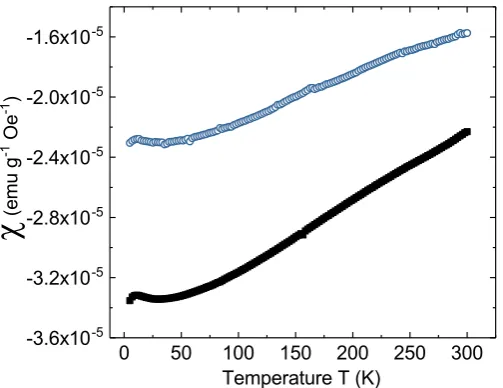
Figure 2.Temperature dependence of the mass susceptibility of two HOPG samples from the same source with thicknesses of 201µm (bottom curve) and 27µm (upper curve) measured with a SQUID magnetometer.
As already reported in the literature, the change of the diamagneticc−axis susceptibility with 151
temperature is rather weak, having a maximal diamagnetic response at∼50 K with a slight increase at 152
lower temperatures, as Figure2shows. The presented result of the bulk sample is similar to published 153
results (see, e.g., Fig. 6 in [32]). The results shown in Figure2indicate that the absolute value of the 154
magnetic susceptibility of the thinner sample is'25% smaller than samples with thickness of 30.6 155
µm or 201µm at 300 K. Having the samples similar areas and prepared from the same bulk sample, 156
this difference is not due to an error in the measurement or because the quality of the sample has 157
been changed through handling. These variations of the susceptibility for similar samples of different 158
thickness (see also Fig.4) already suggest a non-intrinsic origin of the main diamagnetic signal. 159
(B) Angle dependence of the torque:The torque magnetometer can be used to obtain the magnetic 160
moment for one field direction if the sample is strong magnetically anisotropic, i.e.χkχ⊥, where the 161
two susceptibilities mean for fields parallel and perpendicular to thec−axis. According to published 162
results the ratio between the two susceptibilities isχk/χ⊥&10 [1,2,31,33]. This means that the torque 163
-30 0 30 60 90 120 150 180 210 240 -0.03
-0.02 -0.01 0.00 0.01 0.02 0.03
T
o
r
q
u
e
(
a
.
u
.
)
Angle (degree)
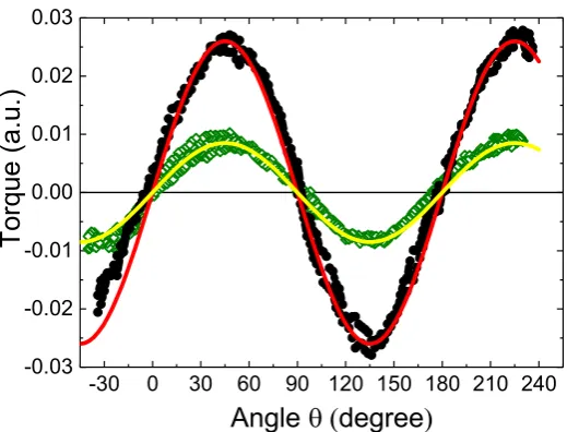
Figure 3.Torque signal of two natural graphite flakes vs. angleθbetween the applied fieldH=2 kOe and thec-axis of the graphite structure. The thickness of the samples was 1.2µm (♦) and 6.9µm (•). The lines are fits to a sin(2θ)function. The magnetic moment of the thinnest sample is of the order of ∼ −2×10⁻⁹emu.
Figure3shows as example the angular dependence of the measured torque signal under a 165
constant magnetic field of 2 kOe at room temperature performed on two different pieces of a natural 166
graphite sample of thickness 1.2µm and 6.9µm. The measurements were done in the two field sweep 167
directions and, as can be seen in the figure, a good reproducibility was achieved with negligible 168
hysteresis. The magnetic moment obtained from the torque signal depends on the angleθbetween the 169
applied magnetic fieldHand thec-axis of the samples, as shown in Figure3. 170
(C) Thickness dependence of the diamagnetic susceptibility: 171
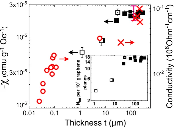
Figure4shows the results of thec−axis susceptibility of all graphite samples we have measured 172
at 300 K as a function of their thickness and with the two experimental methods. In the same figure we 173
included the thickness dependence of the conductivity of graphite obtained at the same temperature 174
(righty-axis) taken from [13,34]. Our data basically agree with the published susceptibility data of 175
highly ordered samples of thickness of the order or larger than 100µm. However, note the variations 176
of± ∼25% (vertical bar in the upper right in the figure) even for similar samples. We observe that 177
when the thickness of the samples is less than∼50µm, dimensional effects begin to appear on the 178
electrical as well as in the magnetic susceptibility of graphite. Fort<50µm the experimental trend 179
suggests a change of a factor of ten in the susceptibility within a change of∼3 orders of magnitude in 180
thickness. This means roughly a change of∼30% in one decade of thickness. Note that all measured 181
susceptibility points have a constant, practically thickness independent background contribution 182
coming from the rest of the graphene (mainly Bernal stacking) layers, see section4. In Appendix A 183
of the supplementary information we show also the behaviour of the resistivity at 4 K as a function 184
of the sample thickness. In Appendix B we demonstrate that the observed decrease of the measured 185
0.01 0.1 1 10 100 3x10 -6 3x10 -5 10 -6 10 -5
1 10 100 2
6 10 14 18
Thickness t (µm)
( e m u g -1 O e -1 ) 10 -2 10 -1 C o n d u ct i vi t y ( 1 0 6 O h m -1 cm -1 ) N i n t p e r 1 0 4 g r a p h e n e p l a n e s
Figure 4.c-axis susceptibility of different graphite samples vs. their thickness at 300K measured by a torquemeter() and a SQUID magnetometer(). The samples were obtained from pre-characterized bulk natural graphite [15] as well as HOPG samples of grade ZYA [13,15,35]. The HOPG sample with a thickness 30.6 µm was measured with the SQUID as well as with torque magnetometer ( , see Appendix D in the supplementary information for details of the calibration of the torque magnetometers). The vertical error bar at the top right indicates the values at 300K reported of different oriented samples in the literature [32,36–41]. Righty-axis: thickness dependence of the conductivity of several bulk and thin graphite samples at 300K from (◦) [13] and (×) [34], calculated using the given geometry in those publications. The inset shows the estimated effective number of interfaces (per 104graphene layers) that contribute to the diamagnetic signal as a function of the sample thickness, obtained using Equation (1).
The observed behavior strongly suggests that the observed internal microstructure of the graphite 187
samples plays a mayor role in those properties. The transport [10,13,14] and structural studies [15] 188
indicate that graphite samples have to be considered, electronically speaking, not as homogeneous but 189
as a heterostructure. In other words, each sample with thickness&20 nm may start showing three 190
contributions to the conductivity as well as to the susceptibility: two semiconducting-like phases with 191
Bernal and rhombohedral stacking orders and some of the interfaces between the semiconducting 192
phases or twisted by a certain angle within the same stacking order [10], with metallic and/or 193
superconducting character [10,13,14,22,23,42]. These three contributions conduct in parallel when the 194
current is applied parallel to the graphite layers. Decreasing therefore the thickness of the sample below 195
a certain thickness, the diamagnetic contribution to the magnetization, given in first approximation by 196
the simple addition of the three magnetic contributions in series, would decrease because the largest 197
contribution proportional to the diamagnetic response of the interfaces would also decrease. 198
4. Discussion 199
The decrease of the absolute value of the susceptibility decreasing the thickness of the ordered 200
graphite samples does not appear to be related to extra defects one may introduce through handling or 201
sample preparation (see also Appendix B and C in the supplementary information). Neither the error 202
in the misalignment between thec−axis and the applied field direction nor the error in the sample 203
dimensions or mass can provide changes of±25% observed in thicker samples or a factor of five in the 204
susceptibility of thinner samples, see Figure4. It should be clear that due to the heterostructure of most 205
semiconducting character of the two stacking orders, the magnetic properties of graphite cannot be 207
explained with the models proposed in the literature [4–6] and new approaches are needed. 208
To understand at least semiquantitatively the observed behavior we take a simple approach, 209
which main aim is to estimate the order of magnitude of the total measured magnetic moment of the 210
samplemassuming that it is due to the direct sum of the independent moments from the 2D interfaces 211
mint, the Bernal (mB) and the rhombohedral(mRH)stacking orders as: m= mint+mB+mRH. The
212
estimates done below provide the order of magnitude and an explanation for the thickness dependence 213
of the total susceptibility. 214
We note that there are neither high-resolution band structure measurements nor calculations 215
especially for the Bernal stacking orders that provide the obtained small energy gap. This is necessary 216
to get the dispersion relation, the Fermi velocity and the effective carrier mass at low enough energy, 217
which eventually can be used to estimate the susceptibility of each of the stacking orders. Therefore, 218
we shall assume that each of those contributions is given by the 2D susceptibility of the graphene 219
layers in each stacking order, similarly for the 2D highly conducting interfaces, multiplied by their 220
corresponding densities. The measured c-axis susceptibilityχ, with the magnetic field Happlied 221
normal to the graphene and interface planes, is estimated as: 222
223
χ=a(χint
Nint
N +χB NB
N +χRH NRH
N ), (1)
224
where the parametersNi(i=int, B, RH)refer to the effective number of interfaces, and the number of 225
graphene layers that belong to the Bernal and rhombohedral phases in a given sample;Nis the total 226
number of layers in a given sample of thicknesst. The prefactorain Equation (1) is a normalization 227
factor inversely proportional to the 2D mass density. It can be roughly calculated or obtained directly 228
from a comparison with the measuredχat large enough thickness. 229
To estimate thec−axis magnetic susceptibility of the two semiconducting phases with energy gaps∼38 meV and∼110 meV we take the formula for the orbital diamagnetic susceptibility of a graphene layer with a band gap∆given by (in cgs units) [43]:
χ∆=−gvgse
2v2
F 6πc2
1
2∆, (2)
wheregs =2 andgv=2 represent the degrees of freedom associated with spin and valley, respectively, andcthe light velocity. We estimate the electron velocityvFfor a 2D electron system as:
vF = }
√ 2πn
m? , (3)
230
wherem?is the effective mass of electrons. From experiments one can obtain a carrier concentration at 231
room temperaturen∼1010cm−2[10,18,22]. With this we estimate a carrier velocityvF ∼3×105cm/s 232
assuming that for these semiconducting phases the effective mass is equal to the free electron mass 233
with a quadratic dispersion relation. Future measurements should clarify the value of the effective 234
mass at least for the majority Bernal phase (without interfaces). The 2D diamagnetic susceptibilities are 235
χB∼ −4×10⁻¹⁷emu/cm2Oe andχRH∼ −10−17emu/cm2Oe, where we used the samenfor both
236
stacking orders. We expect thatχRHshould be even smaller than the estimate above.
237
The 2D diamagnetic susceptibility of the internal interfaces is obtained from the expression 238
for the Landau diamagnetism of a 2D gas of free electrons, taking from experiments the effective 239
mass m? ∼ 0.05me [44,45] (me is the free electron mass). Note that the SdH oscillations in the 240
magnetoresistance are related to the carriers at the interfaces and not to the semiconducting layers. 241
[8–10]. This is obvious because the thinnest, semiconducting samples without interfaces should have a 243
negligible amount of conduction electrons at low enough temperatures [10,14]. 244
The Landau diamagnetic susceptibility of the interfaces is therefore:
χint=−
e2
12πm?c2 ∼ −2×10
−13emu/cm2Oe . (4)
245
246
From STEM studies we know that the ratio of the number of interfaces and of the graphene planes 247
with one or other stacking orders depend on sample and on the position on the same sample, see e.g. 248
[10,15]. Furthermore, although each interface is parallel to the graphene layers, they do not cover 249
all the mesoscopic sample area; they are limited at least within the single crystalline regions with 250
a length and width within a range of∼1 . . . 20µm, as electron backscattering diffraction pictures 251
indicate [46,47]. This means that a single interface covers in general an area much smaller than the one 252
of the graphene planes. As the thickness of the sample decreases, the probability of having similar 253
diamagnetic response due to the effective distribution of 2D interfaces also decreases. In other words, 254
the relative weight of each single interface is in general less than 1 compare to the graphene layers that 255
cover the whole sample area. 256
To estimate the total susceptibility vs. thickness, with the knowledge of the typical thickness of 257
the Bernal and rhombohedral crystalline regions and the number of embedded interfaces obtained 258
from the STEM images, one can roughly estimate an effective ratio of the number of interfaces in a 259
given sample to the number of graphene layers Nint
N . For example and to fix ideas, the following trends 260
are rather general Nint
N (t.50 nm)→0 and Nint
N (t>50µm)∼1.6×10⁻³. The range of the ratio of 261
graphene planes of the Bernal phase is NB
N ∼0.8 . . . 1 and of the rhombohedral NRH
N ∼0.2 . . . 0. 262
This estimate indicates that in real ordered graphite samples with thicknesst & 30 µm and 263
for a typical ratio of the number of interfaces, the total susceptibility is given mainly by the 264
conducting interfaces. Moreover and in first approximation the rhombohedral contribution to the 265
total susceptibility can be neglected. With the estimates given above, using the measured value of 266
the susceptibilityχ(t > 50µm) ∼ −2×10⁻⁵emu/gOe we obtaina∼ 6×1010 cm2/g. From the 267
experimental data and using Equation (1) we estimate the ratioNint/Nvs. the sample thickness, 268
shown as inset in Figure4. 269
Future experiments should try to measure the susceptibility of graphite samples with smaller 270
thickness down to∼ 10 nm and area. 1µm2, because the probability to have the contribution 271
of interfaces is evidently smaller. If these measurements are achieved successfully one can obtain 272
the susceptibility of the Bernal phase and compare with the theoretical model. This susceptibility 273
represents a rather constant background of the experimental points shown in Fig.4. However, the 274
technical difficulties to measure such small samples with the systems available nowadays are difficult 275
to overwhelm. 276
Finally, we would like to pay attention to an actually common observation in the laboratories, 277
when one tries to leave a thin graphite flake completely or partially levitating under an inhomogeneous 278
magnetic field from a permanent magnet. We observed that not all thin flakes react similarly to the 279
same field distribution, even when they have similar mass and shape. Even several of them do not 280
react at all to the magnetic field, independently of how small their mass is. This simple observation 281
already indicates that our simple assumption of a homogeneous diamagnetic response of graphite 282
samples cannot be correct. Within our interpretation these observations can simply indicate that the 283
selected thin samples have different amount of conducting interfaces. 284
Furthermore, an interesting observation was included a year ago in the YouTube internet channel. 285
Namely: large, thin and flat pieces of pyrolytic graphite that levitate on North-South chessboard grid 286
of neodymium magnets can be moved, tilted or shifted by the application of a strong enough laser 287
provoked movement is due to a local decrease of the diamagnetic response in the sample. It would 289
be interesting to measure the temperature of the sample during heating and observe changes in its 290
levitation behavior after crossing a temperature around∼400 K, which is of the order of the critical 291
temperature of the superconducting-like response reported in [15,49]. 292
5. Materials and Methods 293
Samples 294
In order to investigate the magnetization of graphite samples with different thickness, several 295
well-ordered graphite samples were selected taking into account previous characterization with 296
STEM, XRD, magnetotransport and particle induced x-ray emission (PIXE) measurements. The bulk 297
samples were natural graphite samples from Sri Lanka and Brazil [15] as well as HOPG samples of 298
grade A (ZYA) (Union Carbide, Advanced Ceramic and SPI) of very high purity [12,35,50]. The total 299
magnetic impurities concentration of the selected samples was below 3 ppm. See Appendix C in 300
the supplementary information for more details on the results of this characterization as well as the 301
arguments against the speculation that impurities or sample edges are the reason for the observed 302
behavior of the susceptibility. 303
The embedded interfaces can be well recognized through STEM picture on Figure1(see also [10]) 304
and the existence of the two well-ordered stacking orders by XRD [13,15]. 305
To check for the quality of our samples and the reliability the used experimental setup, we 306
measured the diamagnetic response of bulk samples of thicknesst > 50µm with the SQUID and 307
the torque magnetometer. The measuredc−axis mass susceptibility at 300 K of all bulk samples was 308
χ' −(2.2±0.3)×10−5emu/g Oe, in good agreement with previously reported values for highly 309
oriented bulk samples [3,31,37,51]. The mass of the graphite samples was measured with a Mettler 310
Toledo AG245 balance. The size of the samples with thickness larger than 100µm were measured with 311
an optical microscope, otherwise using a SEM. 312
SQUID measurements 313
We have used two different magnetometers, a SQUID and a torque magnetometer; details of this 314
last are given below. The SQUID measurements were done with a SQUID from Quantum Design. The 315
samples were prepared as follows: Precharacterized bulk samples were selected, i.e. HOPG ZYA and 316
natural graphite samples from Sri Lanka and Brazil mines. The HOPG ZYA samples were glued with 317
a small amount of cryogenic vanish to a thin silicon substrate (4×4×0.18 mm3). In Appendix E 318
of the supplementary information we describe further the influence of the substrate on the SQUID 319
measurements. The natural graphite samples obtained from a bulk sample were attached to a long, 320
highly pure quartz rod using a small amount of varnish with thec−axis of the sample parallel to the 321
applied field. The selected samples were exfoliated with a scotch tape in such a way that the surface of 322
the graphite flake was as flat as possible. The background magnetic signals of the silicon substrate, 323
varnish as well as of the quartz rod were previously characterized. They are much smaller (absolute 324
value) than the signal of the samples, see Appendix E in the supplementary information. 325
Finally, the graphite samples with their substrates were placed in a plastic straw keeping the 326
magnetic field direction parallel to the c-axis of the graphite structure within ±2◦. Before each 327
measurement, we left the superconducting solenoid with a remanence below 0.1 Oe, using the 328
oscillating mode option of the SQUID. The magnetization was measured at different fixed fields 329
at 300 K. Afterwords the whole measuring process was repeated. All susceptibility values shown and 330
discussed in this manuscript were obtained at fieldsH6104Oe. 331
Torque measurements 332
Since graphite is a strong anisotropic material [31], its magnetic properties can be also investigated 333
a vacuum system with a water-cooled rotating magnet for the generation of fields up to 4 kOe, 335
an AC Resistor Bridge AVS-47 with preamplifier, a Lake Shore Model 325 Cryogenic Temperature 336
Controller and the torque magnetometer itself. It consists of a piezo-resistive cantilever PRSA-L300 337
from SCL-Sensor. Tech. Fabrication GmbH. The cantilever has 4 piezoresistors in a Wheatstone bridge 338
circuit increasing the sensitivity to magnetic moments of the order ofm∼5×10⁻¹⁰ emu at 1 kOe. 339
The Wheatstone bridge is also used to compensate the magnetic field influence on the piezoresistors. 340
Two resistors are placed at the edge of the cantilever for torque measurements and further two on the 341
cantilever base for current compensation. A picture of the cantilever tip of the two magnetometers 342
with the samples can be see in Figure5. 343
The bulk natural samples were cleaned in ethanol and in an ultrasonic bath for 5 to 7 minutes 344
for purification and a further fragmentation of the bulk piece. Ethanol droplets containing graphite 345
flakes dropped onto a silicone substrate covered by 150 nm silicon nitride layer (Si3N4). Afterwards
346
the samples were dried on the substrates for more than one day and were attached at the edge of the 347
cantilever as shown in Figure5. Before starting the measurements we waited for a stable vacuum and 348
temperature (300 K) for two days. Since the diamagnetic response at fields parallel to thec−axis of 349
highly oriented graphite does not depend strongly on temperature, see Figure2, we restricted the 350
torque measurements to 300 K. 351
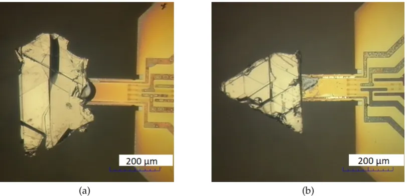
(a) (b)
Figure 5.Natural graphite flakes on the tip of the cantilevers. The sample thickness was (a) 1.2µm and (b) 6.9µm. The other samples dimensions can be taken from the pictures using the scale bar that indicates 200µm. The bent seen in picture (a) does not represent a large portion of the graphite flake but it comes from a small part just at the sample surface. It represents an insignificant contribution to the total sample mass (or volume) affecting less than 1% the absolute value of the susceptibility. This is estimated through side pictures.
A simple way to check the calibration of the torque magnetometers used is to measure sample big 352
enough so that one can measure them also with the SQUID. This has been done with one sample. We 353
have checked the calibration through estimates of the strength factors for each cantilever following [52]. 354
After calibration of the torque signal the susceptibility was calculated dividing the magnetic moment 355
field slope by the mass of the samples. Further details of the original experimental data, calibration 356
procedure and estimates of the spring constant of the cantilevers necessary to calculate the magnetic 357
moment can be read in Appendix D of the supplementary information. To check for the magnetic 358
anisotropy and simultaneously the quality of the samples, the angle dependence of the torque has 359
6. Conclusion 361
Our results show that the absolute value of the diamagnetic susceptibility of highly ordered 362
graphite is not constant, as assumed in the literature, but it depends on the sample even for samples of 363
the same batch and volume. Below a certain thickness, our results indicate a decrease of the absolute 364
value of the diamagnetic susceptibility with the sample thickness. Although more experimental data for 365
thinner samples are needed to completely assure the observed trend, the behavior is compatible with 366
recent studies of the galvanomagnetic properties of graphite. These as well as our results indicate the 367
existence of a non-uniform heterostructure in real graphite samples strongly affecting their magnetic 368
and electrical properties. The presented results stress the need of a reconsideration of previously 369
published models used to understand the magnetic and electrical properties of graphite samples. 370
Supplementary Materials:The following are available online athttp://www.mdpi.com/2312-7481/xx/1/5/s1: 371
Appendix A (Comparison between the thickness dependence of the susceptibility and of the electrical conductivity 372
at 4 K and 300 K) with one figure, Appendix B (Surface to volume ratio) with two figures, Appendix C (Particle 373
induced x-ray emission (PIXE) characterization of the samples impurities), Appendix D (Original experimental 374
data and the calibration curve) with two figures and Appendix E (Influence of substrate on SQUID measurements). 375
Author Contributions:B.S. performed all the magnetic measurements and data curation; P.D.E. performed the 376
supervision of the experimental work; B.S. and P.D.E. conceived and designed the experiments and analyzed the 377
data, and wrote the paper together. 378
Funding:B.S. was supported by Erasmus Mundus Webb project. P.E. was partially supported by the Mincyt from 379
Argentine with the Milstein fellowship during his stay at the Instituto Balseiro in Bariloche, the University of 380
Buenos Aires and the University of Tucumán, where part of the manuscript was written. 381
Acknowledgments: We acknowledge A. Champi and H. Beth for providing us with the natural graphite samples 382
from Brazil and Sri Lanka, and W. Böhlmann for the STEM pictures. B.S. greatly thanks the support of A. 383
Deutschinger, B. C. Camargo, J. Barzola-Quiquia, A. Setzer, V. Zviagin and M. Stiller. 384
Conflicts of Interest:The authors declare no conflict of interest. The funders had no role in the design of the 385
study; in the collection, analysis and interpretation of data; in the writing of the manuscript and in the decision to 386
publish the results. 387
Abbreviations 388
The following abbreviations are used in this manuscript: 389
390
2D two dimensional
HOPG Highly Oriented Pyrolytic Graphite SEM Scanning Electron Microscopy
STEM Scanning Transmission Electron Microscopy SQUID Superconducting Quantum Interference Device 391
392
1. Krishnan, K.S.; Ganguli, N. Large Anisotropy of the Electrical Conductivity of Graphite. Nature1939, 393
144, 667. doi:https://doi.org/10.1038/144667a0. 394
2. Mrozowski, S. Semiconductivity and Diamagnetism of Polycrystalline Graphite and Condensed Ring 395
Systems. Phys. Rev.1952,85, 609–620. doi:10.1103/PhysRev.85.609. 396
3. Heremans, J.; Olk, C.H.; Morelli, D.T. Magnetic susceptibility of carbon structures. Phys. Rev. B1994, 397
49, 15122–15125. doi:https://doi.org/10.1103/PhysRevB.49.15122. 398
4. McClure, J.W. Diamagnetism of Graphite. Phys. Rev.1956,104, 666–671. doi:10.1103/PhysRev.104.666. 399
5. Sharma, M.P.; Johnson, L.G.; McClure, J.W. Diamagnetism of graphite. Phys. Rev. B1974,9, 2467–2475. 400
doi:10.1103/PhysRevB.9.2467. 401
6. Dresselhaus, M.S.; Dresselhaus, G.; Sugihara, K.; Spain, I.L.; Goldberg, H.A.Graphite Fibers and Filaments; 402
Springer Verlag Berlin, 1988. doi:10.1007/978-3-642-83379-3. 403
7. Kelly, B.T.Physics of Graphite; London: Applied Science Publishers, 1981. 404
8. Ohashi, Y.; Hironaka, T.; Kubo, T.; Shiiki, K. Magnetoresistance Effect of Thin Films Made of Single 405
9. Ohashi, Y.; Yamamoto, K.; Kubo, T. Shubnikov - deHaas effect of very thin graphite crystals. Carbon’01,
407
An International Conference on Carbon, Lexington, KY, United States, July 14-19, Publisher: The American Carbon
408
Society2001, pp. available at www.acs.omnibooksonline.com, 568–570.
409
10. Esquinazi, P.D.; Lysogorskiy, Y., Basic Physics of functionalized graphite; Springer Series in Materials 410
Science 244, P. Esquinazi (ed.), Springer International Publishing AG Switzerland, 2016; chapter 7, pp. 411
145–179. doi:10.1007/978-3-319-39355-1. 412
11. Zhang, Y.; Small, J.P.; Pontius, W.V.; Kim, P. Fabrication and electric-field-dependent transport 413
measurements of mesoscopic graphite devices. Appl. Phys. Lett.2005,86, 073104. doi:10.1063/1.1862334. 414
12. Barzola-Quiquia, J.; Yao, J.L.; Rödiger, P.; Schindler, K.; Esquinazi, P. Sample Size Effects on the 415
Transport Characteristics of Mesoscopic Graphite Samples. phys. stat. sol. (a)2008,205, 2924–2933. 416
doi:10.1002/pssa.200824288. 417
13. Zoraghi, M.; Barzola-Quiquia, J.; Stiller, M.; Setzer, A.; Esquinazi, P.; Kloess, G.H.; Muenster, T.; Lühmann, 418
T.; Estrela-Lopis, I. Influence of rhombohedral stacking order in the electrical resistance of bulk and 419
mesoscopic graphite. Phys. Rev. B2017,95, 045308. doi:10.1103/PhysRevB.95.045308. 420
14. Zoraghi, M.; Barzola-Quiquia, J.; Stiller, M.; Esquinazi, P.D.; Estrela-Lopis, I. Influence of interfaces on the 421
transport properties of graphite revealed by nanometer thickness reduction. Carbon2018,139, 1074 – 1084. 422
doi:https://doi.org/10.1016/j.carbon.2018.07.070. 423
15. Precker, C.E.; Esquinazi, P.D.; Champi, A.; Barzola-Quiquia, J.; Zoraghi, M.; Muiños-Landin, S.; Setzer, A.; 424
Böhlmann, W.; Spemann, D.; Meijer, J.; Muenster, T.; Baehre, O.; Kloess, G.; Beth, H. Identification of a 425
possible superconducting transition above room temperature in natural graphite crystals. New J. Phys.
426
2016,18, 113041. doi:https://doi.org/10.1088/1367-2630/18/11/113041. 427
16. Inagaki, M.New Carbons: Control of Structure and Functions; Elsevier, 2000; chapter 2. 428
17. Lin, Q.; Li, T.; Liu, Z.; Song, Y.; He, L.; Hu, Z.; Guo, Q.; Ye, H. High-resolution TEM 429
observations of isolated rhombohedral crystallites in graphite blocks. Carbon2012, 50, 2369 – 2371. 430
doi:https://doi.org/10.1016/j.carbon.2012.01.054. 431
18. García, N.; Esquinazi, P.; Barzola-Quiquia, J.; Dusari, S. Evidence for semiconducting behavior 432
with a narrow band gap of Bernal graphite. New Journal of Physics 2012, 14, 053015. 433
doi:10.1088/1367-2630/14/5/053015. 434
19. Kopnin, N.B.; Ijäs, M.; Harju, A.; Heikkilä, T.T. High-temperature surface superconductivity in 435
rhombohedral graphite. Phys. Rev. B2013,87, 140503. doi:10.1103/PhysRevB.87.140503. 436
20. Muñoz, W.A.; Covaci, L.; Peeters, F. Tight-binding description of intrinsic superconducting correlations in 437
multilayer graphene. Phys. Rev. B2013,87, 134509. doi:https://doi.org/10.1103/PhysRevB.87.134509. 438
21. Scheike, T.; Esquinazi, P.; Setzer, A.; Böhlmann, W. Granular superconductivity at room 439
temperature in bulk highly oriented pyrolytic graphite samples. Carbon 2013, 59, 140 – 149. 440
doi:https://doi.org/10.1016/j.carbon.2013.03.002. 441
22. Ballestar, A.; Barzola-Quiquia, J.; Scheike, T.; Esquinazi, P. Josephson-coupled superconducting regions 442
embedded at the interfaces of highly oriented pyrolytic graphite. New Journal of Physics2013,15, 023024. 443
doi:10.1088/1367-2630/15/2/023024. 444
23. Cao, Y.; Fatemi, V.; Fang, S.; Watanabe, K.; Taniguchi, T.; Kaxiras, E.; Jarillo-Herrero, P. 445
Unconventional superconductivity in magic-angle graphene superlattices. Nature 2018, 556, 43–50. 446
doi:10.1038/nature26160. 447
24. Zoraghi, M.; Barzola-Quiquia, J.; Stiller, M.; Setzer, A.; Esquinazi, P.; Kloess, G.; Muenster, T.; Lühmann, 448
T.; Estrela-Lopis, I. Influence of rhombohedral stacking order in the electrical resistance of bulk and 449
mesoscopic graphite. Phys. Rev. B2017,95, 045308. doi:10.1103/PhysRevB.95.045308. 450
25. Pamuk, B.; Baima, J.; Mauri, F.; Calandra, M. Magnetic gap opening in rhombohedral-stacked multilayer 451
graphene from first principles. Phys. Rev. B2017,95, 075422. doi:10.1103/PhysRevB.95.075422. 452
26. Henck, H.; Avila, J.; Ben Aziza, Z.; Pierucci, D.; Baima, J.; Pamuk, B.; Chaste, J.; Utt, D.; Bartos, 453
M.; Nogajewski, K.; Piot, B.A.; Orlita, M.; Potemski, M.; Calandra, M.; Asensio, M.C.; Mauri, F.; 454
Faugeras, C.; Ouerghi, A. Flat electronic bands in long sequences of rhombohedral-stacked graphene. 455
doi:10.1103/PhysRevB.97.245421. 456
27. Kuwabara, M.; Clarke, D.R.; Smith, A.A. Anomalous superperiodicity in scanning tunnelling microscope 457
28. Miller, D.L.; Kubista, K.D.; Rutter, G.M.; Ruan, M.; de Heer, W.A.; First, P.N.; Stroscio, J.A. Structural 459
analysis of multilayer graphene via atomic moiré interferometry. Phys. Rev. B2010, 81, 125427. 460
doi:https://doi.org/10.1103/PhysRevB.81.125427. 461
29. Flores, M.; Cisternas, E.; Correa, J.; Vargas, P. Moiré patterns on STM images of graphite 462
induced by rotations of surface and subsurface layer. Chemical Physics 2013, 423, 49–54. 463
doi:http://dx.doi.org/10.1016/j.chemphys.2013.06.022. 464
30. Brihuega, I.; Mallet, P.; González-Herrero, H.; de Laissardière, G.T.; Ugeda, M.M.; Magaud, L.; 465
Gómez-Rodríguez, J.M.; Ynduráin, F.; Veuillen, J.Y. Unraveling the Intrinsic and Robust Nature of 466
van Hove Singularities in Twisted Bilayer Graphene by Scanning Tunneling Microscopy and Theoretical 467
Analysis.Phys. Rev. Lett.2012,109, 196802. doi:https://doi.org/10.1103/PhysRevLett.109.196802. 468
31. Fischbach, D.B. Diamagnetic susceptibility of pyrolytic graphite. Phys. Rev. 1961, 123, 1613–1614. 469
doi:10.1103/PhysRev.123.1613. 470
32. Tongay, S.; Hwang, J.; Tanner, D.B.; Pal, H.K.; Maslov, D.; Hebard, A.F. Supermetallic conductivity in 471
bromine-intercalated graphite. Phys. Rev. B2010,81, 115428. doi:10.1103/PhysRevB.81.115428. 472
33. Kopelevich, Y.; Esquinazi, P.; Torres, J.H.S.; Moehlecke, S. Ferromagnetic- and Superconducting-Like 473
Behavior of Graphite. Journal of Low Temperature Physics2000,119, 691–702. doi:10.1023/A:1004637814008. 474
34. Iye, Y.; Tedrow, P.M.; Timp, G.; Shayegan, M.; Dresselhaus, M.S.; Dresselhaus, G.; Furukawa, A.; Tanuma, S. 475
High-magnetic-field electronic phase transition in graphite observed by magnetoresistance anomaly. Phys.
476
Rev. B1982,25, 5478–5485. doi:10.1103/PhysRevB.25.5478.
477
35. Spemann, D.; Esquinazi, P.; Setzer, A.; Böhlmann, W. Trace element content and magnetic properties of 478
commercial HOPG samples studied by ion beam microscopy and SQUID magnetometry.AIP Advances
479
2014,4, 107142. doi:https://doi.org/10.1063/1.4900613. 480
36. Krishnan, K.S. Magnetic Anisotropy of Graphite. Nature1934,133, 174?175. doi:10.1038/133174c0. 481
37. Ganguli, N. Magnetic studies on graphite and graphitic oxides. The London, Edinburgh, and Dublin
482
Philosophical Magazine and Journal of Science1936,21, 355–369. doi:10.1080/14786443608561589.
483
38. Fischbach, D.B. Diamagnetic Susceptibility of Pyrolytic Graphite. Phys. Rev. 1961,123, 1613–1614. 484
doi:10.1103/PhysRev.123.1613. 485
39. Simon, M.D.; Geim, A.K. Diamagnetic levitation: Flying frogs and floating magnets (invited). Journal of
486
Applied Physics2000,87, 6200–6204,[https://doi.org/10.1063/1.372654]. doi:10.1063/1.372654.
487
40. Sepioni, M.; Nair, R.R.; Rablen, S.; Narayanan, J.; Tuna, F.; Winpenny, R.; Geim, A.K.; Grigorieva, 488
I.V. Limits on Intrinsic Magnetism in Graphene. Phys. Rev. Lett. 2010, 105, 207205. 489
doi:10.1103/PhysRevLett.105.207205. 490
41. Miao, X.; Tongay, S.; Hebard, A.F. Extinction of ferromagnetism in highly ordered pyrolytic graphite by 491
annealing. Carbon2012,50, 1614 – 1618. doi:https://doi.org/10.1016/j.carbon.2011.11.040. 492
42. Ballestar, A.; Esquinazi, P.; Böhlmann, W. Granular superconductivity below 5 K in SPI-II pyrolytic graphite. 493
Phys. Rev. B2015,91, 014502. doi:10.1103/PhysRevB.91.014502.
494
43. Koshino, M.; Ando, T. Singular orbital magnetism of graphene. Solid State Communications2011,151, 1054 – 495
1060. doi:https://doi.org/10.1016/j.ssc.2011.05.012. 496
44. Soule, D.E.; McClure, J.W.; Smith, L.B. Study of the Shubnikov-de Haas Effect. Determination of the Fermi 497
Surfaces in Graphite.Phys. Rev.1964,134, A453–A470. doi:10.1103/PhysRev.134.A453. 498
45. Williamson, S.J.; Foner, S.; Dresselhaus, M.S. de Haas-van Alphen Effect in Pyrolytic and Single-Crystal 499
Graphite. Phys. Rev.1965,140, A1429–A1447. doi:10.1103/PhysRev.140.A1429. 500
46. González, J.C.; Muñoz, M.; García, N.; Barzola-Quiquia, J.; Spoddig, D.; Schindler, K.; Esquinazi, 501
P. Sample-Size Effects in the Magnetoresistance of Graphite. Phys. Rev. Lett. 2007, 99, 216601. 502
doi:https://doi.org/10.1103/PhysRevLett.99.216601. 503
47. García, N.; Esquinazi, P.; Barzola-Quiquia, J.; Ming, B.; Spoddig, D. Transition from Ohmic to ballistic 504
transport in oriented graphite: Measurements and numerical simulations. Phys. Rev. B2008,78, 035413. 505
doi:10.1103/PhysRevB.78.035413. 506
48. Magnetic Games. https://www.youtube.com/watch?v=cJx5rAuXIXQ&list=PLigZQCghm_vwGEtIBnOfCLEm485_l1K8f. 507
49. Stiller, M.; Esquinazi, P.D.; Barzola-Quiquia, J.; Precker, C.E. Magnetic Force Microscopy Measurements 508
of Superconducting Permanent Current Paths in a Natural Graphite Crystal. J. Low Temp. Phys. 2018, 509
50. Spemann, D.; Esquinazi, P.D., Evidence for Magnetic Order in Graphite from Magnetization and Transport 511
Measurements. InBasic Physics of Functionalized Graphite; Esquinazi, P.D., Ed.; Springer International 512
Publishing: Cham, 2016; pp. 45–76. doi:10.1007/978-3-319-39355-1_3. 513
51. Miao, X.; Tongay, S.; Hebard, A.F. Extinction of ferromagnetism in highly ordered pyrolytic graphite by 514
annealing. Carbon2012,50, 1614 – 1618. doi:https://doi.org/10.1016/j.carbon.2011.11.040. 515
52. Cleveland, J.P.; Manne, S.; Bocek, D.; Hansma, P.K. A nondestructive method for determining the spring 516
constant of cantilevers for scanning force microscopy. Review of Scientific Instruments1993,64, 403–405. 517