University of South Carolina
Scholar Commons
Theses and Dissertations
8-9-2014
Three Essays on Consumer Product Returns
Guangzhi Shang
University of South Carolina - Columbia
Follow this and additional works at:https://scholarcommons.sc.edu/etd
Part of theBusiness Administration, Management, and Operations Commons
This Open Access Dissertation is brought to you by Scholar Commons. It has been accepted for inclusion in Theses and Dissertations by an authorized administrator of Scholar Commons. For more information, please [email protected].
Recommended Citation
Three Essays on Consumer Product Returns
by
Guangzhi Shang
Bachelor of Business Administration The Hong Kong Polytechnic University 2010
Submitted in Partial Fulfillment of the Requirements
for the Degree of Doctor of Philosophy in
Business Administration
Darla Moore School of Business
University of South Carolina
2014
Accepted by:
Michael R. Galbreth, Major Professor
Mark E. Ferguson, Committee Member
Pelin Pekgün, Committee Member
Bikram P. Ghosh, Committee Member
c
Dedication
I dedicate this dissertation to my parents,
Dingyu Sun and Yuzhuo Shang,
who have always loved and supported me.
I could not be who I am today without their most generous encouragement.
I also dedicate this dissertation to my grandparents,
Yanhua Hui, Shuwen Shang, Cuihua Jiang, and Longjia Sun,
who give me the warmest smiles that lighten up my life,
Acknowledgments
I give my first thanks to my advisor, dissertation chair, and coauthor, Dr. Mike
Galbreth. I feel extremely lucky that my interaction with Mike started very early in
my PhD career. Mike taught me step-by-step about how to develop an interesting
idea into a research project. His caring and patient personalities are precious treasures
for me because I often find myself obsessed with experimenting with thoughts that do
not materialize into concrete ideas. I’m deeply indebted to him for having the kind
of freedom that a doctoral student can rarely enjoy. I am extremely happy that this
flexibility helped me take the most difficult yet essential course for a young researcher,
in my opinion. That is, how to learn things outside classroom and on demand. I have
to also thank him for giving me endless encouragements, especially during some of
the low times.
My next big thanks goes to Dr. Mark Ferguson, my dissertation committee
mem-ber, mentor, and program director. I wish I could have the opportunity to work
with Mark even earlier. He gave me many inspirations of how to spice up academic
research with more practicality. I went to my first practitioners’ conference with him,
where I found out nerdy research can also be easy-going. Being the PhD program
director, Mark provided me with the most generous travel funding, which was the life
blood for a student who often needs to spend beyond his budget.
I would also like to thank my other dissertation committee members, Dr. Bikram
Ghosh and Dr. Pelin Pekgün. I learned many analytical skills from Bikram during
working on a project that he was very generous to have me involved. Pelin has the
an attribute that I certainly need more development in my career. My dissertation
could not have come this far without the support from all of you. Thanks again!
Let me also give my gratitude to Dr. Manoj Malhotra for his guidance on two
other projects and his help as a recommender. I need also to thank Dr. Sanjay Ahire
for his generosity of providing help in the early stage of this dissertation. I also want
to mention Dr. Stephen Finger, who have taught my industrial organization class
and born with my endless questions on econometrics.
I would like also to thank my coauthors on various projects, not previously
men-tioned, Dr. Joan Donohue, Dr. Timothy Fry, and Dr. Robert Ployhart. I also want
to acknowledge those professors who have either directly taught me or indirectly
inspired me.
My previous officemates and good friends, Dr. Cidgem Ataseven, Dr. Ashley
Metcalf, and Dr. Mariana Nicholae, have given me so much fun during my PhD
study. My current officemates and good friends, Erin McKie, Minseok Park, Cherry
Singhal, Deepa Wani, and Övünç Yılmaz, have provided me with some thoughts on
my dissertation and cared for my well-being in the program. Julia Witherspoon,
our department secretary, and Scott Ranges, our business PhD program coordinator,
have answered my numerous questions regarding the administrative duties. A big
thanks to them as well.
I want to also thank all my friends at University of South Carolina, who influenced
me in some way. Although it’s impossible to list all of them, those come to mind
include Nicholas Bailey, Ruiyuan Chen, Wen Chen, Yin Fu, Hye Sun Kang, Chris
Ling, Pulkit Nigam, He Wang, Yijia Zhao, and Dr. Xiaolan Zheng.
The last and most special thanks go to my girlfriend Shengfang Sun, who I shared
Abstract
Return policies (aka. money-back-guarantee policies) are frequently offered by
retail-ers such that consumretail-ers can bring back the purchased products that do not fit their
needs. On the benefit side, consumers perceive these policies as a risk-mitigation
service and are willing to pay more for an otherwise identical product. All else being
equal, being lenient in its return policy should allow a retailer to enjoy higher sales,
which leads to increased revenue. On the cost side, a generous return policy will
in-duce more returns and possibly also late returns. In 2007 alone, U.S. manufacturers
and retailers paid more than $100 billion to process consumer returns. For electronic
products, this cost is estimated at $16.7 billion per year, which represents 6% of an
average electronics manufacturer’ revenue and 3% of an average retailer’s total sales.
The return rate in the retail sector ranges from 10% to 20%. To effectively manage
returns, a retailers should concurrently optimize its price and restocking fee so that
it could enjoy the most benefit from offering a return policy. At the same time, it
should also seek to better forecast the quantity of incoming returns and make efforts
to reduces the number of futures returns.
Despite the magnitude of the returns management problem, academic research on
this topic is still relatively scant. Through three separate studies, this dissertation
delves into returns management from a multitude of perspectives. The first study
explores a retailer’s optimal return policy when a fraction of the market is consist of
opportunistic consumers, who might purchase with the explicit intention of returning.
The second study demonstrates how retailers might use their point-of-sale data to
identify products that are more likely to be returned. The last study introduces
a novel approach for retailers to quantify the incremental willingness-to-pay that
Table of Contents
Dedication . . . iii
Acknowledgments . . . iv
Abstract . . . vi
List of Tables . . . xi
List of Figures . . . xiii
Chapter 1 Overview . . . 1
Chapter 2 Return Policies with Consumer Opportunism . . . 4
2.1 Introduction and Literature . . . 4
2.2 Model . . . 6
2.3 Results . . . 9
2.4 Extension: Linking Salvage Value to the Benefit of Opportunism . . . 16
2.5 Conclusion . . . 17
Chapter 3 Returns Forecasting and Retailer Practices . . . 19
3.1 Introduction . . . 19
3.2 Literature Review . . . 22
3.4 Data and Variables . . . 28
3.5 Return Forecasting . . . 34
3.6 Managerial Implications . . . 45
3.7 Conclusion . . . 50
Chapter 4 Value of a Money-Back-Guarantee Policy . . . 52
4.1 Introduction and Literature . . . 52
4.2 Decomposing the Value of an MBG policy . . . 57
4.3 Data and Variables . . . 62
4.4 The Econometric Model . . . 67
4.5 Analysis and Results . . . 74
4.6 Conclusion . . . 84
Chapter 5 Future Research . . . 88
Bibliography . . . 90
Appendix A Proof of Lemma 2.1 . . . 97
Appendix B Proof of Proposition 2.1 . . . 101
Appendix C Proof of Proposition 2.2 and Corollary 2.1 . . . 102
Appendix D Proof of Proposition 2.3 . . . 103
Appendix E Proof of Proposition 2.4 . . . 104
Appendix G Finite Sample Performance of the Estimators . . . . 107
List of Tables
Table 3.1 Descriptive Statistics of Product Categories . . . 29
Table 3.2 Descriptive Statistics of Independent Variables . . . 35
Table 3.3 Description of Period-Level Data . . . 36
Table 3.4 Description of Period-Level Data in Replication Samples . . . 36
Table 3.5 Average Forecast Accuracy Improvements . . . 42
Table 3.6 Estimation Results . . . 44
Table 3.7 Time Windows Equivalent to 95th Percentile of Experience Du-ration . . . 47
Table 3.8 Average Marginal Effects . . . 48
Table 4.1 Money-Back-Guarantee Policies of On-line Consumer Electron-ics Retailers . . . 54
Table 4.2 Difference in Consumer Valuation Between MBG and No-MBG Transactions . . . 64
Table 4.3 Summary Statistics for the Shipping Fee Variable . . . 66
Table 4.4 Descriptive Statistics . . . 68
Table 4.5 Estimation Results . . . 73
Table 4.6 Likelihood Ratio Tests . . . 76
Table 4.7 The Value of MBGs by Seller Cluster . . . 79
Table 4.8 Robustness Checks . . . 82
Table 4.10 Estimates of MBG Value by Category . . . 87
Table A.1 Retailer Profit Function (Main Model) . . . 97
Table A.2 Optimal Return Policies (Main Model) . . . 98
Table E.1 Optimal Return Policies When Salvage Value Linked to Benefit
of Opportunism . . . 105
Table F.1 Model Specification for Two-week and One-month Cases . . . 106
Table G.1 Finite Sample Performance of OLS, 2SLS, and FIML Estimators . 109
List of Figures
Figure 2.1 Retailer’s Optimal Return Policy Regions . . . 10
Figure 2.2 Impact of the Extent of Opportunism on Optimal Profit . . . 12
Chapter 1
Overview
Consumer product returns represent a substantial challenge and a size-able expense
for retailers and manufacturers. In 2007 alone, U.S. manufacturers and retailers paid
more than $100 billion to process consumer returns Blanchard (2007). For electronic
products, the cost of returns in the U.S. has been estimated at $16.7 billion per
year, representing 6% of revenue for an average consumer electronics manufacturer
and 3% of total sales for an average retailer (Douthit et al., 2011). According to
National Retail Federation (2011a), the return rate in the retail sector ranges from
10% to 20%. Despite such magnitude, research on the management of consumer
returns is relatively scant. This dissertation attempts to delve into three critical and
intriguing issues for managing returns. The key insights are previewed in following
three paragraphs.
Most retailers offer refunds to consumers who, after a trial period, return a product
that they find does not fit their needs. There is evidence from practice that some
consumers are willing to use this return option opportunistically, essentially “renting”
a product by using it during the trial period and then returning it. Restocking fees
(partial refunds) can be used to combat this behavior. However, such fees might be
viewed negatively by consumers in cases where the return is due to a true lack of fit.
We derive optimal pricing and return policies that explicitly consider both the extent
of opportunism (how many consumers consider such behavior) and the benefit of
opportunism (the attractiveness of the renting option). Our analysis reveals several
present in the marketplace. We also examine the profit impact of changes in the
extent or benefit of opportunism, finding that this impact is not always intuitive, and
that increases in either of these two opportunism constructs can actually increase
profits in some cases. In an extension, we provide additional insights for when the
salvage value of returned items is linked to how much utility has been extracted by
the opportunistic consumer.
Almost all prescriptive practices for lowering the cost of processing returns require
a forecast of how many consumer returns will arrive in each period. Despite the
fact that retail transactions data is readily available and has been shown to provide
significantly better demand forecasts for new product sales, this data has not been
explored for forecasting consumer returns. Using a data set provided by a major U.S.
retail chain and consisting of 20,801 transactions of 2,483 electronic products, we
develop an econometric model that simultaneously explains the consumer’s experience
duration and return probability, which is in turn used for predicting return quantity
in a given time period. This approach yields 20% to 40% lower forecast errors than
the benchmark time-series models, and the performance gain is sustained even with a
very parsimonious set of explanatory variables. Our econometric model also identifies
promising managerial actions for lowering the cost of consumer returns such as better
targeting of buyer assistance programs and choosing different return time windows
for specific product families.
While Money-Back-Guarantee (MBG) return policies are common in practice, the
academic literature provides little guidance on the value, if any, that consumers assign
to such a policy. For on-line retailers, both shipping charges and seller reputation
may influence the perceived value of MBGs. A non-refundable forward shipping
charge is likely to be perceived by consumers as an implicit restocking fee and hence,
decrease the value of an MBG policy. On the other hand, good customer feedback
eyes of consumers. To investigate the value of MBGs in the on-line context, we
collect the final selling prices of identical products offered by different vendors (with
different return policies) on eBay auctions. Our data set includes 2946 transactions
across 86 consumer electronic products. Endogeneity of the MBG decision by sellers
is addressed using a maximum likelihood estimator based on the error correlation
structure. We estimate that offering an MBG policy for on-line consumer electronics
increases a customer’s valuation of a product by an average of 5.2% and show that this
increase is substantially influenced by both seller reputation and shipping charges.
Our results provide an empirical measure of the value of an MBG that can be weighed
Chapter 2
Optimal Retail Return Policies with Consumer
Opportunism
2.1 Introduction and Literature
Returns are viewed as necessary by many retailers since it is often impossible for a
consumer to fully resolve all uncertainty regarding the fit of the item to her needs
before a purchase is made (Nelson 1970). In-store assistance, on-line reviews, and
other resources can provide some information, but a trial period is often needed
to assess fit. Indeed, Ferguson et al. (2006) explain that products are often returned
with no functional or cosmetic defect, but rather because a mismatch between product
attributes and consumer preferences is revealed during the trial period. Reasons for
mismatch can include installation difficulty, product performance issues, or remorse
(Kumar et al., 2002). Given the role of the trial period in resolving fit uncertainty,
it is generally accepted that consumers should have the opportunity to return a
non-defective retail purchase for a refund (possibly net of a restocking fee) if, after further
evaluation, they find that it does not meet their needs. However, consumer returns are
not driven exclusively by product mismatch with consumer needs – some consumers
take advantage of lenient return policies by purchasing items with the explicit intent
of returning them after a period of use, essentially “renting” the items. Familiar
examples of such opportunistic behavior include buying a digital camcorder to use
on a single vacation or buying a cocktail dress to wear to one event. This type of
customers (McWilliams, 2004), while studies of apparel retailers have dubbed the
behavior “wardrobe borrowing” (Wood, 2001). According to a recent survey by the
National Retail Federation (2011b), 61.4% of retailers experience such opportunistic
returns.
Most analytical models of consumer returns assume that no consumers will
con-sider opportunistic behavior (e.g. Su, 2009; Shulman et al., 2011; Hsiao and Chen,
2012; Akçay et al., 2013). On the other hand, a few studies have assumed that all
consumers will consider opportunistic behavior (Chu et al., 1998; Hess et al., 1996).
We suggest that the best representation of reality lies between these two extremes.
Specifically, since opportunistic behavior is not consistent with the intention of the
returns policy, it may be viewed as socially unacceptable by some consumers (indeed,
casual conversations about this research have elicited responses ranging from open
admissions of opportunistic behavior to expressions of outrage at the idea).
Will-ingness to consider such actions is a function of one’s psychological traits such as
self-concept (Mazar and Ariely, 2006) and symbolic self-completion (Rosenbaum and
Kuntze, 2005). Laboratory evidence has shown that individuals who emphasize the
alignment between self-image and social desirability will not engage in
opportunis-tic behavior (Mazar et al., 2008). Thus, a model of returns behavior should reflect
the fact that some consumers reject opportunistic behavior while others include it
in their consideration set. Accordingly, in this study we assume that there exists an
exogenous fraction of consumers who will consider opportunistic returns behavior.
We use the analytical framework of Su (2009) (see also Akçay et al., 2013) to
model a retail context in which returns might occur due to a low realized valuation
of the product once uncertainty has been eliminated after purchase. We augment
this framework to accommodate the coexistence of two consumer segments - an
“op-portunistic” segment (willing to consider renting items) and an “ordinary” segment
is conceptualized as having two components: the size of the opportunistic segment
(which we refer to as the extent of opportunism), and the fraction of product value
that can be extracted by opportunistic consumers during the trial period (the
ben-efit of opportunism). In the following sections we examine the impact of these two
opportunism constructs on the retailer’s optimal pricing strategy and profits.
2.2 Model
We consider a monopoly retailer selling to a market consisting of some mix of
op-portunistic and ordinary consumers. We first delineate how each segment makes its
purchase and subsequent keep/return decisions. We then determine the resultant
demand from each segment and derive total retailer profits.
Consumers
The products of interest for our analysis are experience goods (Nelson, 1970). At the
time of purchase, consumers face uncertainty regarding whether an experience good
will match their needs. This uncertainty will be resolved after product trial. Following
the approach of Su (2009) and Akçay et al. (2013), we assume that consumers have
the sameex ante evaluation of the product, v0, and their ex post adjustments to this
initial evaluation, ε, are random draws from a common distribution. Specifically,
we let v0 = 12 and ε uniformly distributed between −12 and 12. Put it differently,
consumers’ true evaluation of the product, v = v0 + ε, is uniformly distributed1
between 0 and 1.
As described in the Introduction, consumers in our model are categorized into
two groups based on their willingness to opportunistically use the return policy to
1The assumption that a consumer’s post-trial product evaluation follows a uniform distribution
rent a product. Ordinary consumers use the product trial period for its intended
purpose — to assess fit. They do not consider renting, as they find this behavior to
be inconsistent with social norms and thus unacceptable. Opportunistic consumers
do not find renting unacceptable, either because it is accepted by their social peers
or because they have a low regard for social desirability (Mazar and Ariely, 2006;
Mazar et al., 2008). Note that opportunistic consumers do not simply use the trial
period to asses fit - instead, they use the product intensively during the trial period,
and hence their returns might be in worse condition than returns made by ordinary
consumers. We denote size of segment of opportunistic consumers, i.e. theextent of
opportunism, as γ. It follows that rest of the market, 1−γ, is made up of ordinary
consumers.
Each consumer makes two decisions: first, she decides whether or not to buy
the product; secondly, after realizing her true valuation of the product, she decides
whether to keep or return it. Assuming a pricep and a restocking feef, an ordinary
consumer who has purchased will keep the product if her realized product evaluation,
v, is at least as high as the refund, p−f. If the opposite is true (v < p−f), she will
return the product and claim the refund. Thus, her expected net utility from making
the purchase is Uor =Emax(v, p−f)−p. Uor can be simplified as follows:
Uor =Emax(v, p−f)−p= Z 1
p−f
vdv+
Z p−f
0
(p−f)dv−p= 1 + (p−f)
2−2p
2 (2.1)
Opportunistic consumers consider abusing the return policy such that they
par-tially consume the product during the trial period and pay the restocking fee.
Es-sentially, this abusive behavior is analogous to renting from the retailer, where rental
period is the return time window and rental charge is the restocking fee. Letβdenote
the fraction of product value consumed before return, β ∈ [0,1]. It follows that the
rent option gives opportunistic consumers βv+p−f utility. That is, the sum of the
consumed product value, βv, and the refund, p−f. We refer to β as the benefit of
tuxedo versus a casual jacket. The former is typically used on rare occasions, while
the latter is intended for everyday wear. In other words, a larger proportion of the
value of a tuxedo can be consumed in just a few uses, as opposed to the much slower
consumption of a casual jacket. Thus, ceteris paribus, the tuxedo has a much higher
β than the casual jacket (a similar example of the product-specific nature of β was
observed in the experimental study of Hjort and Lantz (2012)). The same logic
ap-plies for many other product categories – camcorders vs. music players, sunglasses
vs. eyeglasses. etc. – in which some items might be needed for use on specific,
rare occasions (such as a camcorder or sunglasses on a vacation) while others provide
recurring benefits over a longer period of time.
For the opportunistic segment, a consumer who has purchased the product
com-pares the utilities of renting, βv+p−f, and keeping,v, to decide whether to make
an opportunistic return. The two options have the same utility whenv = 1p−−fβ. When
β is large, i.e. 1p−−fβ >1, it is possible that opportunistic consumers will always return.
In this case, their expected net utility from purchasing the product Uop is simply
E(βv+p−f)−p. If β is small and hence p1−−fβ ≤1, their expected net utility Uop is
Emax(v, βv+p−f)−p instead. Uop can be simplified as follows:
Uop=
Emax(v, βv+p−f)−p= 1−β+(f2(1−p)−2β−)2p(1−β) for 1p−−fβ ≤1,
E(βv+p−f)−p= 2β −f for p1−−fβ >1.
(2.2)
We restrict our attention to γ ∈ [0,12], which essentially states that there are
more ordinary consumers than opportunistic consumers in the market2. If a
prod-uct is returned by an ordinary consumer, the retailer earns restocking fee f plus
salvage value s1 net unit product cost c, i.e. f +s1 −c. If returned by an
oppor-tunistic consumer, the retailer earns f +s2 −c instead. s1 > s2 captures the fact
2National Retail Federation (2011a) reports that fraudulent returns, which nest abusive returns
that opportunistic returns are in worse condition due to excessive wear and tear. In
addition, we assume that 12 > c > s1, which implies that the retailer’s unit product
cost is less than consumers’ average product evaluation but larger than unit salvage
value. Lastly, when a buyer retains her purchase, the retailer earns p − c.
De-note the retailer’s unit profit from ordinary consumers as πor. Given the respective
probabilities of keeping the product, 1−(p−f), and returning it, p−f, we have
πor = (p−c)[1−(p−f)] + (f+s1−c)(p−f). Denote the unit profit from
opportunis-tic consumers as πop1 for p1−−βf < 1 and πop2 for p1−−βf > 1. Recall that when p1−−fβ <1,
some opportunistic consumers return, and when p1−−fβ >1, all opportunistic consumers
return. Thus we haveπop1 =
1− p−f
1−β
(p−c) +p1−−fβ(f+s2−c) andπop2 =f+s2−c.
Normalizing the market size to 1, the retailer’s profit function is as follows.
π=
(1−γ)πor+γπop1 for p1−−fβ ≤1,
(1−γ)πor+γπop2 for p1−−fβ >1.
(2.3)
The retailer’s problem is to choose the pricepand restocking feef that maximize
(2.3) subject to the constraints that both segments of consumers participate in the
market (Uor ≥0, Uop≥0).3 The timing of the game is as follows:
1. The retailer chooses the price p and restocking feef.
2. Consumers make their purchases and realize their true valuations v.
3. Ordinary consumers keep the product if v > p−f and return it otherwise;
opportunistic consumers keep the product ifv > βv+p−fand return otherwise.
2.3 Results
Solving the retailer’s optimization problem yields the following lemma:
3In Appendix A, we show that it is always profit maximizing for the retailer to serve both
segments as long as a mild condition on unit product cost ,c < M in[1−s1+2s21
2 ,
2s2+s21(−1+s2(2+s2))
4s2 ],
Figure 2.1 Retailer’s Optimal Return Policy Regions
Lemma 2.1. The retailer’s optimal price (p∗) and restocking fee (f∗) depend on the
extent (γ) and the benefit (β) of opportunism, which together define three regions of
the solution space. Table A.2 in Appendix A summarizes p∗, f∗, and optimal profit
(π∗), as well as the boundary conditions for each region. Figure 2.3 provides a visual
illustration of the three optimal policy regions (c= 0.35, s1 = 0.3, and s2 = 0.15 in
that figure).
Note that when there is no opportunistic consumer (γ = 0), our optimal price
(p∗ = 1+s21
2 ) and restocking fee (f
∗ = (1−s1)2
2 ) are consistent with previous literature
(Akçay et al., 2013; Su, 2009) given the uniform distribution of v. Next, we provide
rationale for why the retailer should adopt three distinctive types of return policies.
First, consider the difference between Case I and the other two cases. The benefit
of opportunism,β, captures the opportunistic consumers’ incentive to rent the
prod-uct. Whenβ is low, it is relatively easy to induce opportunistic consumers to keep the
product, since the benefit of renting is relatively low. As β increases, the appeal of
that the probability of keep for the opportunistic segment is 1− p−f
1−β). Consequently,
the opportunistic segment will always rent when β is sufficiently high - this occurs
in Cases II and III in the Figure. The difference between Cases II and III can be
understood as follows. Since opportunistic consumers always rent in these regions,
the only way for the retailer to earn more profit from the opportunistic segment is
through increasing restocking fee, which is evident in πop2 = f +s2 −c. in Case II
(highβ, lowγ), such a restocking fee increase is possible for the retailer. However, as
γ increases, an increasingly large restocking fee is needed to address the prevalence
of opportunism. At some point, a γ threshold is reached - the sum of restocking fee
and salvage value has become very high relative to price - and it is no longer optimal
to continue to increase the restocking fee. This defines Case III (high β, highγ) - as
long as the retailer is in this region, its price and restocking fee are unaffected by γ.
Impact of the Extent of Opportunism
In this section, we study the profit maximizing response to changes in the extent of
opportunism.
Proposition 2.1. (a) Optimal price is non-increasing in the extent of opportunism.
(b) Optimal restocking fee is non-decreasing in the extent of opportunism.
(c) Moreover,
∂p∗
∂γ ≤
∂f∗
∂γ .
We discuss parts (a) and (b) of the Proposition in terms of the regions of the
solution space (Cases I-III) shown in Figure 2.3. First, consider restocking fee. In
Case I and Case II, the retailer should, as expected, always increase restocking fee in
response to more opportunistic consumers. For reasons explained earlier, the retailer
does not adjust restocking fee when both the benefit and extent of opportunism are
Figure 2.2 Impact of the Extent of Opportunism on Optimal Profit
extract more profit from the opportunistic segment, it needs to decrease price at the
same time in order to offset this cost for ordinary consumers.
The intuition for part (c) follows from this idea of an offsetting price decrease
along with the fact that, at optimality, an ordinary consumer’s probability of keeping
the product is always larger than the probability of returning it. Thus, the negative
utility impact of increased restocking fee can be offset by a price decrease of a lesser
magnitude (since the probability of incurring the price is larger than the probability
of incurring the restocking fee).
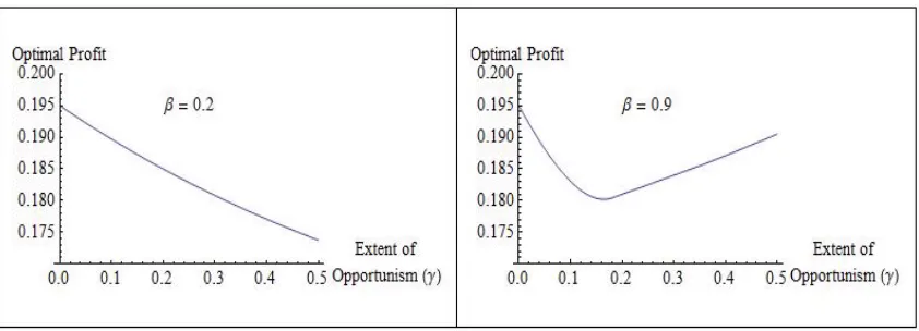
Proposition 2.2. (a) When the benefit of opportunism is low (β <βb), optimal profit
is decreasing in the extent of opportunism, γ.
(b) When the benefit of opportunism is high (β > βb), optimal profit is U-shaped
in the extent of opportunism, γ. βb= √
(s1−s2)(9s1−s2)+s2 2s1 −
1 2.
Figure 2.3 provides a visual illustration of the above proposition (c= 0.35, s1 =
0.3, ands2 = 0.15 in that figure). To more clearly explain this finding, we decompose
the profit impact of the extent of opportunism into three parts, ∂π∂γ∗ = ∂[(1−γ)π
∗
or+γπ∗op]
∂γ =
(1−γ)∂πor∗
∂γ +γ ∂πop∗
∂γ + (π
∗
op−πor∗ ). The first two parts measure the indirect effects of
γ transmitted by the segment-specific unit profits, while the last part measures the
from zero, the retailer gradually shifts the focus of its pricing scheme away from the
ordinary segment, evidenced by raising the restocking fee. Therefore, it is intuitive
to see that the unit profit it earns from the ordinary segment is decreasing (∂πor∗
∂γ <
0), while its unit profit from the opportunistic segment is increasing (∂π
∗
op
∂γ > 0).
Interestingly, we can show that the weighted average of these two counteracting
unit-profit effects, (1 − γ)∂π∗or
∂γ + γ ∂πop∗
∂γ , is always zero. It follows that the final effect
of γ – a certain number of ordinary consumers is replaced by the same number of
opportunistic consumers – determines overall effect of γ on optimal profit.
Since the unit profit from ordinary consumers (π∗or) is always decreasing in the
extent of opportunism and that from the opportunistic consumers (πop∗ ) is always
increasing, π∗op−πor∗ increases in γ. That is, switching an opportunistic consumer
with an ordinary one is more costly to the retailer when the extent of opportunism
is small. As γ increases, πop∗ −πor∗ continues to raise. However, whether this negative
effect can change its sign and turn to a positive one depends on the profitability of the
opportunistic consumers. When the benefit of opportunism (β) is high, opportunistic
consumers are willing to pay a high price to rent the item, which implies that the
retailer is able to profit more from the returns through a high restocking fee. Indeed,
we see that optimal profit can increase with the the opportunistic segment size only
when β is high.
To summarize, opportunistic consumers are always detrimental to the retailer’s
profit when renting is relatively less attractive to them (lowβ). However, when these
consumers can extract more benefit from renting (high β) and hence become more
profitable to the retailer, an increase in the opportunistic segment has a
counter-intuitive U-shaped effect on retailer’s profit. In other words, an increase in the extent
of opportunism can increase profits in some cases.
Corollary 2.1. When optimal profit is decreasing in the extent of opportunism, it
decreases at a decreasing rate. That is, ∂∂22πγ∗ >0 given
∂π∗
The above finding makes an interesting practical implication for retailers.
Con-sider the technologies available for identifying individuals who make return claims
at abnormally frequent rates, such as the Verify-2 by Retail Equation Inc. (Speights
and Hilinski, 2005). Employing such tracking technologies, retailers can marginally
reduce the number of opportunistic consumers, γ. Now, assume a retailer’s is in the
region where its profit is negatively affected by γ. Corollary 2.1 provides guidance
into when the marginal benefit of adopting the technology is highest. Specifically, we
find that a reduction in the opportunistic segment size provides the largest payoff
when size of the segment is small. Therefore, when informed by this result, retailers
should adopt a more proactive approach toward combating abusive returns. In other
words, the best timing for investing in the returns tracking technology is,
counter-intuitively, not when the opportunistic consumer population is considerable but when
it is still limited.
Impact of the Benefit of Opportunism
We now turn our attention to the second aspect of consumer opportunism - the
benefit of opportunism,β. Note that retailers might have some limited influence over
βthrough adjusting the time duration of the return window – longer windows provide
more opportunity to benefit from an item before returning it. Thus, β is analogous
to γ in the previous section in that, while neither is a firm’s decision variable, both
might be influenced at the margin (β by adjusting the return time window, γ by
implementing consumer tracking technologies). This limited endogeneity makes the
following comparative statics particularly relevant.
Proposition 2.3. The marginal impact of the benefit of opportunism (β) on profit,
∂π∗
∂β, can be either zero or positive or negative:
(a) Optimal profit is unaffected by βforβ ∈[1−s1,1]andγ ∈[0, M in[γ,b
β+s1−1 2β+s1−1]].
(c) Optimal profit is decreasing in β otherwise. γ =M ax[ (s1−s2)(−1+β)
s2−s1(1−β)−2s2β,
β+s1−1 2β+s1−1].
In comparing Proposition 2.3 with 2.2, it is interesting to note that, while both β
andγ can be considered as measures of the potential negative impact of opportunism,
they affect profit in different ways. Specifically, an increase in the benefit of
oppor-tunism, β, has a more nuanced impact – it could be either beneficial or irrelevant
or detrimental to retailer’s profit. Since β to a certain extent is controlled by the
time length of return window, Proposition 2.3 offers interesting insights into when
and how a longer return window exerts an indirect effect on retailer’s profit.
When the extent of opportunism is relatively low (part (a) of Proposition 2.3),
the retailer tailors its return policy more towards the ordinary segment through a low
restocking fee. This low restocking fee, if coupled with a high benefit of opportunism
β, induces the opportunistic consumers to always rent. As long as γ is low, it is not
optimal for the retailer to combat this renting through a higher restocking fee, which
would discourage the ordinary consumers (who make up most of the market) from
buying. As a result, the retailer simply maintains a “static” return policy in this
region (no changes to p or f) as β increases. This explains, in part (a) of the above
proposition, why β has no impact on optimal profit when β is high and γ is low.
Next, we consider part (b), where both γ andβ are high - i.e. many opportunistic
consumers deriving a large utility from renting. In this context, the retailer can tailor
its return policy more towards the opportunistic segment, which is relatively large
and has a high valuation of the rental option. Asβ increases further, renting becomes
even more appealing, and the retailer can aggressively raise restocking feef and enjoy
a higher unit profit from the opportunistic segment. The higher restocking fee does
deter ordinary consumers, but the increased profits from the opportunistic segment
more than offset this loss, and the net result is that profits increase.
Lastly, increases in the benefit that consumers receive from opportunistic behavior
β increases the frequency of abusive behavior in the opportunistic segment. If the
restocking fee is also lenient, the retailer cannot recover the lost of net sales due to an
increased volume of returns. This is exactly what happened in part (c) of the above
proposition.
2.4 Extension: Linking Salvage Value to the Benefit of Opportunism
In the previous section, we make the reasonable assumption that an item returned
by an opportunistic consumer will have a lower salvage value than one returned by
an ordinary consumer. In this section, we refine this aspect of the model by explicitly
linkingβ to salvage value. Recall that ordinary consumers simply use the trial period
to assess the fit of the product to their needs, while opportunistic consumers use the
product intensively during the trial. By definition, higher-βproducts can be used more
intensively by opportunistic consumers during the trial, and thus might show more
signs of wear-and-tear than lower-β products, in turn leading to a lower salvage value
(lowers2). As mentioned earlier, that a longer time window increases the opportunity
to extract value during the trial period (higher β). In this section we consider the
possibility that it might also lead to a lower salvage value of opportunistic returns.
Our model can be changed to reflect this by simply redefining s1 = s and s2 =
s−βδ. With this setup we retain model parsimony while capturing the idea that
a higher β increases the quality differential between the opportunistic returns and
the ordinary returns. At the same time, s2 is still strictly smaller than s1, which
preserves the expectation that renting in general reduces salvage value relative to
product evaluation by an ordinary consumer. Details of the analysis of this extension
is in Appendix E. We find that, while all of our previous insights regarding the extent
of opportunism (γ) remain valid, the profit impact of the benefit of opportunism (β)
Proposition 2.4. When salvage value is linked to β, the marginal impact of β on
profit, ∂π∂β∗, can be either positive or negative:
(a) Optimal profit is increasing in β for β ∈[s2+δδ,1] and γ ∈[δβ(1(s−−βδ)),12].
(b) Optimal profit is decreasing in β otherwise.
Proposition 2.4 differs from Proposition 2.3 when γ is low and β is high (this
context is included in part (b) of Proposition 2.4). When salvage value is linked to
the benefit of opportunism, β exerts a negative impact on profit. This contrasts with
the finding of no profit impact of β in this context with the main model (part (a)
of Proposition 2.3). Recall that when the opportunistic segment size is small, the
retailer implements a low restocking fee. When this low γ is coupled with a high
incentive to rent (highβ), it is optimal (in both the main model and this extension)
for the retailer to, in essence “write off” the opportunistic consumers and maintain
a “static” return policy with respect to β (optimal price and restocking fee do not
change with β). Thus, the expected profit from an opportunistic consumer in the
main model is f∗+s2 −c , while it is f∗+s−βδ−c in this extension. Therefore,
when γ is low and β is high, further increments in β will have a negative impact on
firm profit when salvage value is linked to the benefit of opportunism.
2.5 Conclusion
This chapter contributes to the retail operations literature by incorporating the
be-havior of opportunistic consumers into a retailer’s optimal return policy decisions.
By incorporating two opportunism-related constructs, extent and benefit of
oppor-tunism, into our analytical framework, we provide several counter-intuitive and novel
managerial insights. We first demonstrate that the monopolistic retailer’s optimal
response to an increased number of opportunistic consumers is not always to increase
the restocking fee. When the extent of opportunism is low but the benefit of
that when a restocking fee is necessary, it should always be accompanied by a price
decrease of a smaller magnitude.
My analysis of the profit impact of the extent of opportunism confirms the
com-mon expectation that an increase in consumer opportunism will hurt firm profits,
but only when the benefit of opportunism is low. By examining the second order
effects, we refine this conventional wisdom by showing that an increase in the extent
of opportunism has the most detrimental impact on profits when the segment of
op-portunistic consumers is currently small. More interestingly, we also show that, if the
retail context involves both a high benefit and a high extent of opportunism, the
re-tailer’s optimal profit can actuallyincreasewith the size of the opportunistic segment.
This implies that actively working to reduce opportunism might not increase profits
in certain business contexts. Lastly, our analysis of impact of changes in the benefit
of opportunism reveals that its profit impact can be zero, positive, or negative, and
we define the conditions under which each of these is the case. These results suggest
that there are there are cases in which the firm might actually prefer to increase the
Chapter 3
Using Transactions Data to Improve Consumer
Returns Forecasting and Retailer Practices
3.1 Introduction
In 2010, electronics retailer Best Buy eliminated its 15% restocking fee for consumer
electronics. By offering a more lenient return policy, Best Buy was aligning itself with
the majority of U.S. retailers. Walmart, for example, has long offered a 90 day full
refund policy for most of its products. One consequence of such lenient policies is that
consumer returns, i.e. items that are returned to the retailer for a full refund during
the allowable time window, represent a significant cost in the supply chain1. They
also present significant operational challenges for both OEMs and retailers, including
how to process and transport returned items, how to staff returns centers, and how
to recover value from returned products via new or existing sales channels.
In the Operations Management area, previous research on consumer returns has
addressed the retailer’s inventory replenishment policy (Ketzenberg and Zuidwijk,
2009), a retailer-manufacturer incentive alignment program designed to reduce the
number of consumer returns (Ferguson et al., 2006), the OEM’s consumer return
allo-cation strategy between selling as refurbished and using for warranty demand (Pince
et al., 2013), and network design for consumer returns (Guide et al., 2006). The
models presented in these papers all share a common element: the requirement of
1According to a study by Douthit et al. (2011), the cost of consumer returns is between 5%
a forecast of the flow of consumer returns. Toktay et al. (2003) report that many
companies rely on simple heuristics for these forecasts, such as multiplying the
pro-jected sales by the historical return rate of a product. Our conversations with over
fifteen OEMs during the 2013 Consumer Returns Annual Conference reveal that this
remains the most common choice2. The returns forecasting literature also provides
little guidance for the consumer returns problem, as it is primarily focused on
fore-casting the flow of end-of-use/end-of-life returns, for which an OEM might use past
sales history to project returns at the end of the product’s useful life. For consumer
returns, however, retailers often have a potentially powerful resource for predictive
modeling – transaction-level data, which typically contains detailed product and price
information and, potentially, each individual consumer’s previous purchase and
re-turn behavior. Despite the fact that retail transactions data is frequently shared with
OEMs for forecasting new product sales (Aviv, 2007), we are not aware of it being
applied to returns forecasting.
Our first contribution in this study is that we explore the power of
transaction-level retail data to improve the accuracy of consumer returns forecasting. In doing
so, we make a contribution to the theory of returns forecasting by addressing two
econometric challenges specific to the behavior of consumers in a retail return context.
First, consumers differ in how certain they are about their valuations of a product
before they make a purchase. During the trial period (i.e. return time window), each
consumer sufficiently experiences the product and adjusts her valuation accordingly,
and the scale of this adjustment is likely to be larger for those with more initial
uncertainty. This heterogeneous nature of trial uncertainty makes incorporating
non-constant error variance necessary. Secondly, consumers also differ in how long it takes
them to sufficiently experience a given product. Of course, the retailer cannot observe
2In fact, none of the OEMs we talked to suggest that their returns forecasting is conducted with
this duration for the products that are not returned, so the only available data on
trial duration is for the products that are returned. Any estimation based solely
on this “selected” sample introduces bias. We address both of these methodological
challenges by constructing an econometric model that simultaneously accounts for
non-constant error variance and sample selection bias.
Our second contribution is that we use our econometric results to provide
guid-ance for retailers’ consumer returns management. Some retailers have attempted to
actively influence the volume of consumer returns through buyer assistance programs
and/or by adjusting the return time window. The goal of the former is to reduce the
probability of a return by helping customers locate the most suitable product, while
the latter is meant to reduce both the number and average age of returns. For buyer
assistance programs, the cost justification depends heavily on: 1) where a product is
in its life-cycle and thus how familiar consumers are likely to be with it, and 2) how
product assortment causes consumers to be less certain about their product choices.
Our model enables us to empirically investigate the affect of these two factors on
the probability that a product will be returned, and thus to suggest some guidance
regarding the focus of buyer assistance. For the return time window, retailers often
set a single policy uniformly across all returns, e.g. 30, 60, or 90 days after the day
of purchase. This rule-of-thumb approach, while simple to understand by consumers,
ignores the fact that some products take longer to evaluate than others. Using our
econometric model we empirically investigate the relationship between product type
and the length of time required for customers to determine their post-purchase utility.
Using data provided by a major U.S. consumer electronics retailer, we apply our
econometric model to 20,801 transactions of 2,483 products. A summary of our
main results is as follows. First, our causal model based forecasting approach is, on
average, 20% to 40% more accurate than a variety of benchmark models that do
sustained even when only month and category dummy variables are included, which
constitutes a very parsimonious and widely available set of explanatory variables.
Second, we provide guidance for buyer assistance programs by showing how factors
such as product variety and product maturity are correlated with the probability of
a product being returned. These findings enable retailers to better allocate scarce
resources within their buyer assistance programs. Third, we provide guidance for
setting the return time windows by deriving a set of reference policies based on our
finding that different types of products require different lengths of time for consumers
to sufficiently experience them and make an assessment of fit. Finally, we empirically
validate the assumption made in Shulman et al. (2009, 2011) that trial uncertainty
is convexly decreasing in product variety.
3.2 Literature Review
Our study is closely related to two emerging literature streams, managing consumer
returns and product returns forecasting. In the first stream, most previous studies
have an analytical focus on deriving the optimal return policies under different
cir-cumstances. Examples include Akçay et al. (2013), Shulman et al. (2009, 2011), and
Su (2009), as well as the model presented in the last chapter. The current study
empirically tests one key assumption made in this literature – that more product
variety leads to lower trial uncertainty. On the empirical side, Anderson et al. (2009)
contrasts an econometric model that incorporates consumer’s buy-return sequential
decisions to the conventional purchase incident model. They demonstrate how the
model could be used to estimate the optional value of a full refund policy. Petersen
and Kumar (2009) hypothesize and empirically confirm that consumers’ past return
volume links positively to their future purchase volume. In a different context, Griffis
et al. (2012) show that consumers who returned in the past tend to order more
never returned. Our research extends this line of discourse by demonstrating that past
return behavior is a also good predictor of future return behavior. Thus, customers
with past returns may not be as profitable as previously conjectured.
The return forecasting literature has a predominant emphasis on end-of-use
re-turns. Toktay et al. (2003) provide a comprehensive review of these studies. While
Toktay et al. (2000) examine the case of Kodak’s single-use cameras, Clottey et al.
(2012) expand on this work by considering alternative distributions for the return
lag. Li et al. (2011) apply count regression techniques to forecast trade-in returns in
a business-to-business context. Despite this extensive literature on end-of-use returns
forecasting, to our knowledge the problem of forecasting consumer returns has not
been addressed in the literature. In contrast to OEMs, who typically have only
aggre-gated period-level sale and return data available, retailers often collect
transaction-level data through Point-of-Sale (POS) technologies and loyalty programs, resulting
in a rich data set for returns forecasting. While not their main focus, Hess and
May-hew (1997) is the only work that shows potential of utilizing transactions data to
predict consumer returns flow. Specifically, they use price and product category to
estimate, for each transaction, the probability of a return and the time lag until a
return. We take the additional step to aggregate these two pieces of information into
a forecast of consumer returns flow (discussed in detail in Section 3.5). Furthermore,
our econometric model can be viewed as a more flexible model that includes Hess
and Mayhew (1997) as a special case, and we show the forecasting capability of both
approaches. While our full econometric model generates 20% to 40% more accurate
forecasts than traditional time-series forecasting techniques, their approach captures
3.3 The Econometric Model
Consider a consumer who purchases an experience product from a retailer, which
is recorded by the retailer as transaction i. Before purchasing the product, assume
the consumer’s utility of the product is µi +vi, where µi is common knowledge to
both the consumer and the retailer, whilevi is the consumer’s private knowledge, not
observed by the retailer. The product trial, i.e. the post-purchase product evaluation
by the consumer, is modeled as follows. Afteryi days of experiencing the product, the
consumer adjusts her utility byτi such that her post-trial utility is di =µi+vi+τi.
There are multiple reasons that the trial uncertainty, or the variance of the trial
experience, V(τi), might vary across transactions. First V(τi) should be larger when
a product is in the early stages of its life-cycle, since publicly available product
in-formation such as consumer reviews becomes more abundant as a product matures.
Second,V(τi) should be larger when there are fewer competing products, since a lack
of alternatives makes it more difficult for a consumer to ascertain whether a product
is the best fit for her needs (Shulman et al. 2009, 2011). Third, V(τi) should be
larger when transactions occur during the holiday season (November and December),
since products purchased during this time are more likely to be gifts and evaluating
what others might like is more difficult than choosing the best product for oneself.
Fourth, there could be category-specific variations in trial uncertainty, since products
in different categories (televisions, cameras, computers, etc.) are quite different in
terms of how easily and accurately their fit can be assessed. We elaborate on the
above points further in Section 3.4 and test each one empirically in Section 3.6.
Note that bothviandτiare not observable to the retailer so they will collapse into
a single error term in estimation. We denote the collapsed error by εi and assume
it follows a normal distribution with first and second moments equal to 0 and σ2
i.
The transaction specific variance, σi2, allows us to explicitly model the heterogeneity
cost of a return, which includes both the restocking fee and any perceived return
hassle. If di − ri > 0, the consumer keeps the purchased item. If di − ri < 0,
she returns it to the retailer. Hence, whether or not a product is returned can be
modeled using a heteroskedastic probit regression. Since only full refunds appear
in our data, ri degenerates into a constant term that captures perceived hassle of
return. In estimation, this constant collapses with the constant in µi, so we drop ri
to simplify notation3. The retailer records the consumer’s return behavior through a
binary variable Ii,Ii = 1 for returns and Ii = 0 for non-returns.
Next, we turn to the duration of experience,yi. We make the common assumption
that it follows a Weibull distribution4. Let y
i =λiui, whereui is a standard Weibull
distributed error term with duration dependence parameterζandλiis a scale function
that allows experience duration to depend on exogenous factors such as product
category and seasonality. This setup of yi is referred to as Accelerated Failure Time
(AFT) in the survival analysis literature. Strictly speaking, yi is the consumer’s
private knowledge, but the retailer may approximate yi using the time lag between
purchase and return.
Since experience duration is observed only when an item is returned, estimating
the parameters in λi using only return transactions may result in biased estimates.
This issue is called non-random sample selection bias (Heckman, 1979), which arises
due to the correlation betweenεi andui. We do not havea priori expectation on the
directionality of this bias because there are reasonable arguments for both positive
and negative correlation. For example, consumers who face “buyer’s remorse” might
be more likely to return the product and also be more likely to end the product trial
early (a positive correlation between εi and ui). On the other hand, a perfectionist
3Price is already included inµ
i. A restocking fee variable could also be included inµi if this fee
varies across transactions.
4Clottey et al. (2012) apply an exponential distribution, which nests within Weibull as a special
might spend a long time testing the product, while her perfectionism might also cause
even small mismatches between her expectations and the product’s functionality to
result in a product return (a negative correlation between εi and ui). Thus, to
obtain consistent estimates, we simultaneously modelyianddiand, more importantly,
explicitly incorporate their conditional correlation.
Note that the conventional setup of a sample selection model that utilizes a
bi-variate normal distribution is not appropriate for our context because we need one
marginal distribution of the bivariate distribution to be Weibull. Previous research
of non-normal selection models, such as the pioneering work by Lee (1983), uses
cop-ula theory to construct flexible bivariate distributions. We adopt a simple form of
the Farlie-Gumbel-Morgenstern copula family (Kotz et al., 2004; Smith, 2003). The
bivariate probability density function (PDF) is as follows:
fy,d(yi, di) =fy(yi)fd(di){1 +θ[2Fy(yi)−1][2Fd(di)−1]} (3.1)
The marginal PDFs are fy(yi) = (yζi)(yλii)ζe
−(yi
λi) ζ
and fd(di) = σ1iφ(di−σiui). The
marginal Cumulative Distribution Functions (CDFs) are Fy(yi) = 1 −e
−(yi
λi) ζ
and
Fd(di) = Φ(diσ−ui
i ) whereθ measures the correlation betweenyi and di and falls in the interval−1< θ <1.
The above specification has three appealing features. First, θ has the same
directional interpretation as the more familiar Pearson’s correlation coefficient, ρ.
That is, a positive θ means that realizations of yi and di on the same side of their
respective medians will appear more frequently, whereas a negative θ indicates a
higher chance of yi and di appearing on the opposite side of their respective
me-dians. In addition, the transformation from θ to ρ is fairly straightforward. ρ =
θ
R
Fy(yi)[1−Fy(yi)]dyi
R
Fd(di)[1−Fd(di)]ddi
√
V ar(yi)V ar(di)
. Second, selection models derived from the FGM
copula family have been reported to have a reasonable speed of convergence in
esti-mation (Boehmke et al., 2006; Prieger, 2002). Third, when applied to duration data,
outperform Lee (1983) approach, where a transformed bivariate normal distribution
is used (Prieger, 2002).
With the bivariate distribution on hand, we can now construct the likelihood
function. The commonly used two-stage estimator presented in (Heckman, 1979) is
not applicable to our problem because the regression equation for yi is not linear in
λi (Lee, 1983). Instead, we develop a Full Information Maximum Likelihood (FIML)
estimator. The retailer confronts two types of data: (1) an item is not returned
(Ii = 0) and (2) an item is returned (Ii = 1) yi days after purchase. The likelihood
of observing the first type is given by
Pr(Ii = 0) = Pr(di >0) = Pr(εi >−µi) = Φ(
µi
σi
) (3.2)
The likelihood of observing the second type is obtained by integrating the joint density
function fy,d(yi, di) over the relevant range of di.
Pr(Ii = 1, yi) = Pr(εi <−µi, yi) = Z 0
−∞fy,d(yi, di)ddi (3.3)
= fy(yi)Φ(−
µi
σi
){1 +θ[1−Φ(−µi
σi
)][2Fy(yi)−1]}
= (ζ yi
)(yi λi
)ζe−(λiyi) ζ
Φ(−µi
σi
){1 +θΦ(µi σi
)[1−2e−(yiλi) ζ
]}
Taking Equation 3.2 and 3.3 together, we are able to describe the log likelihood of
observing the whole sample as follows:
lnL=
n X
i=1
{(1−Ii) ln[Pr(Ii = 0)] +Iiln[Pr(Ii = 1, yi)]} (3.4)
The FIML estimator produced by maximizing Equation 3.4 is asymptotically
consis-tent. Its finite sample performance is examined through a Monte Carlo simulation,
which is available upon request. Within the framework of our simulation, we find the
estimator to have little bias and to produce estimates considerably closer to the true
3.4 Data and Variables
As an effort to promote quality empirical research, the Institute for Operations
Re-search and the Management Sciences (INFORMS) encourages scholars to publish
unique and comprehensive data sets. The outcomes of this effort include a hotel
book-ing data set (Bodea et al., 2009) and a multiechelon supply chain data set (Willems,
2008) published in Manufacturing & Service Operations Management, as well as a
durable consumer electronics data set in Marketing Science (Ni et al., 2012) . Four
features of the last data set make it especially appealing for applying our econometric
model. First, studies of experience goods are often conducted in the context of
con-sumer electronics (see Gu et al. (2012) and Obloj and Capron (2011) for examples).
Second, our model requires transaction-level data, and Ni et al. (2012) suggest that
theirs is, by far, the most comprehensive data set of consumer electronics transactions
available. Third, researchers are specifically encouraged to work on product return
issues with the Ni et al. (2012) data5. Lastly, and perhaps most importantly, the
retailer in this data set employs a extremely generous time window policy for returns
– the longest return lag in the data is 251 days, and there are several others that took
place more than 150 days after purchase. Such leniency in the return time window
permits estimating consumers’ experience duration without truncation issues.
The original data contains 173,262 transactions provided by a major U.S.
elec-tronics chain, the identity of which, for confidentiality reasons, is not provided. All
returns at this retailer are accepted open-box and given a full refund. The
transac-tions in this data set took place between December 1998 and November 2004. We have
limited our attention to the subset of the original data that is applicable to our
con-text. Information goods (CDs, DVDs, books, etc.), accessories (SD cards, batteries,
cords, etc.), and services were excluded since these are fundamentally different from
5More information could be found at the journal’s websitewww.informs.org/Community/ISMS