A T-Matrix Solver for Fast Modeling of Scattering from Multiple PEC Objects

A T-Matrix Solver for Fast Modeling of Scattering from Multiple

PEC Objects

Lin E. Sun*

Abstract—T matrix characterizes the scattering property of a single PEC object and does not depend on the incidence. In this work, we propose a method to derive a reduced-order T matrix for a single 3D PEC object with arbitrary shape. The method is based on the vector addition theorem and the conventional EFIE, MFIE or CFIE methods. Given the T matrix for a PEC object, the scattered fields can be directly calculated from any incidence. For multiple objects, a matrix equation system is built based on the T-matrix and the position of each object. Finally, numerical examples show the accuracy and efficiency for solving the scattering of both spherical and non-spherical arrays. Compared to the moment methods, the computational cost of solving the final matrix equation is reduced by several orders of magnitude.

1. INTRODUCTION

Modeling of electromagnetic scattering from multiple objects has been studied over many years. The popular solutions for analysis of scattering from conducting objects are the finite difference method (FDM), finite element method (FEM) and moment method (MOM). Among the moment methods, electric field integral equation (EFIE), magnetic field integral equation (MFIE) and combined field integral equation (CFIE) with RWG basis functions are widely used. However, for a large problem that includes multiple PEC objects, there are some challenges for the conventional methods. First, it is well known that fast algorithms need to be applied to these methods in order to solve large-scale problems. Second, as the mesh is refined for large problems, the condition numbers of EFIE and CFIE formulations grow fast and can cause the ill-conditioned system matrices. MFIE has a well-conditioned formulation, while it can only be applied to closed objects and is ill-conditioned for interior resonance problems.

The T-matrix method is firstly discussed in [1] for solving electromagnetic scattering problems. Later, [2] extends the T-matrix method to an arbitrary number of scatterers. The total T-matrix is expressed in terms of the individual T-matrices by an iterative procedure. In order to reduce the computational cost of the total T-matrix, a recursive algorithm is proposed in [3–5]. Since then, the use of this idea for various structures has been demonstrated [9–11, 13]. Although a great deal of work has been performed on solving scattering problems of multiple objects using the T-matrix method [12, 14, 15], applying the method to the multiple PEC structures with arbitrary shapes, especially to non-spherical structures is sill limited. Among the literature work for solving the scattering electromagnetic fields from the 3D multiple objects, most of the previous work handles multiple spherical or cylindrical objects only.

In this paper, a method based on T-matrix is proposed to analyze the scattering from multiple PEC objects. In this method, we first discuss how to obtain the T-matrix for each PEC object and

Received 6 April 2018, Accepted 18 July 2018, Scheduled 30 July 2018 * Corresponding author: Lin E. Sun ([email protected]).

then convert it into a small matrix. Then based on the small T-matrix for each object, an algorithm considering the interactions of multiple scatterers is proposed. There are three main advantages of this method. First is that since the T-matrix for each 3D PEC object with arbitrary shape can be found to be very small, the dimension of the system matrix equation for multiple objects can be several orders of magnitude smaller than those from the method of moments. Hence, the computational cost for multi-scatterer problems is greatly reduced compared to the conventional methods. Secondly, the proposed method is not limited to the spherical objects and can be applied to any multiple PEC problems with arbitrary shapes. Finally, since the T-matrix for each object is independent of incidence, the recalculation for difference incidences can be avoided.

2. FACTORIZATION OF THE DYADIC GREEN’S FUNCTION BY VECTOR ADDITION THEOREM

A dyadic Green’s function in EM can be written as

G(r_j,r_i) =

I+∇∇

k2

g(r_j,r_i) (1)

It can be expanded by vector wave functions in spherical coordinates [6, 7]

G(r_j,r_i) =ik ∞

l=1

l

m=−l

1

l(l+ 1)[Mlm(k,rjs)gMˆlm(k,ris))

+N_lm(k,r_js)gNˆ_lm(k,r_is))] (2)

wherer_j−r_i =r_js−r_is,|r_js|<|r_is|. M_lm and N_lm are vector wave spherical harmonics expressed in terms of spherical Hankel functions and spherical harmonics. g means taking the regular part of the function where the spherical Hankel function is replaced by a spherical Bessel function:

M_lm(k,r) =∇ ×rψ_lm(k,r)

N_lm(k,r) = 1

k∇ × ∇ ×rψlm(k,r) (3)

Here,ψ_lm(k,r) is the solution of the Helmholtz equation in free space, and

ψ_lm(k,r) =h(1)_l (kr)Y_lm(θ, φ) (4)

Here,h(1)_l (kr) is the first-kind spherical Hankel function,

Y_lm(θ, φ) =

(l−m)!(2l+ 1) (l+m)!4π P

m

l (cos(θ))eimφ (5)

whereP_lm(x) is the Legendre’s polynomial.

In the above, g means taking the regular part of the function, which means that the spherical Hankel function is replaced by the spherical Bessel function.

gMˆ_lm(k,r) =∇ ×rψˆ_lm(k,r)

gNˆ_lm(k,r) = 1

k∇ × ∇ ×r

_ψˆ_{lm(k,r) (6)}

Here,

ˆ

ψ_lm(k,r) =j_l(kr)Y_lm∗ (θ, φ) (7)

where j_l is the l-order spherical Bessel function. Since Y_lm(θ, φ) is orthonormal, Y_l,−m(θ, φ) = (−1)mY_lm∗ (θ, φ).

Truncating the summation at l = lmax, then the number of terms involved in Eq. (2) is P = (lmax+ 1)2−1. Therefore, Eq. (2) can be rewritten in a more compact form

whereψt(r_js) and gψˆ(r_is) are matrices composed of ordered M_lm and N_lm.

In Eq. (2),M_lm and N_lm can be further expanded by the vector theorem in spherical coordinates [7], that is

M_lm(r) = l_,m

[gM_lm(r)A_lm,lm(r) +gN_lm(r)B_lm,lm(r)]

N_lm(r) = l_,m

[gN_lm(r)A_lm,lm(r) +gM_lm(r)B_lm,lm(r)] (9)

wherer=r+r and|r|<|r|has been assumed.

Next, Substituting Eq. (9) into Eq. (2), we obtain the expansion form for the dyadic Green’s function

G(r_ji) =ik ∞

L_L 1

l(l+ 1)[gML(k,rjs)AL,L(rss)gMˆL(k,ris)

+gN_L(k,r_js)A_L,L(r_ss)gNˆ_L(k,r_is)

+gM_L(k,r_js)B_L,L(r_ss)gNˆ_L(k,r_is)

+gN_L(k,r_js)B_L,L(r_ss)gMˆ _L(k,r_is)] (10)

It can be further written as

G(r_ji) =ik ∞

L_L 1

l(l+ 1)

gM_L(k,r_js)

gN_L(k,r_js)

_T

·

A_L,L(r_ss) B_L,L(r_ss)

B_L,L(r_ss) A_L,L(r_ss)

·

gMˆ _L(k,r_is)

gNˆ_L(k,r_is)

(11)

Here, we use r_js = r_js +r_s,s, where |r_js| < |r_ss|. In the above, L = (l, m), L = (l, m). The expressions forA_lm,lm and B_lm,lm can be found in [7].

In the above, Equation (9) can be written in the compact form as below

ψt(r)3×2P =gψt(r)3×2P ·α(r)2P×2P (12)

When |r|<|r|is assumed, it is written as

ψt(r)3×2P =ψt(r)3×2P ·β(r)2P×2P (13)

whereα and β are translation operators defined in [6, 7].

The expansion of the dyadic Green’s function can also be rewritten in the compact form as

G(r_j,r_i) =gψt(r_js)3×2P ·α(rss)2P×2P · gψˆ(ris)2P×3 (14)

Here, ψt and gψˆ are matrices composed of orderedgM_lm and gN_lm. α is the matrix stacked by

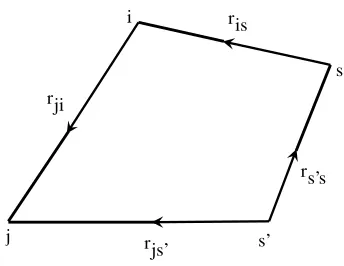
A_L,L and B_L,L. The detailed formulations can be found in Appendix D of [7]. Fig. 1 shows all the position vectors mentioned above.

3. DERIVATION OF THE T-MATRIX FOR A SINGLE PEC SCATTERER

The scattering solution of a PEC object is known as

Es(r) =iωμ

G(r,r)·J(r)dr (15)

To get the scattering solution, usually the PEC object is discretized into RWG basis, and the scattering field of the whole object is discretized into the scattering solution from each basis. Suppose that the PEC object is discretized into M RWG bases, then

Es(r) = M

i=1 iωμ

si

j

i

s’

s r ji

r is

r s’s

r js’

Figure 1. Configuration of position vectors.

Substituting Eq. (1) into Eq. (16) and using the property of the RWG basis, we can get

Es(r) = M

i=1 iωμ

si

g(r,r_i)Λ_i(r_i)dr_i·a_i+ M

i=1 i ω

si

∇g(r,r_i)∇·Λ_i(r_i)dr_i·a_i (17)

Equation (17) is the familiar expression for EFIE equation. Rewrite (r−r) as (r−r_i)−(r_i−r_i) in Eq. (16), and by using the expansion of dyadic Green’s function in Eq. (8), Eq. (16) can be expanded into

Es(r) = M

i=1

ψt(r−r_i)·M_ii·a_i (18)

whereM_ii is defined as

M_ii=iωμ

Si

gψˆ(r_i−r_i)·Λ_i(r_i)dr_i (19)

In the above, r_i denotes the center of thei-th RWG; r_i are the sampling points on the RWG; a_i is the current coefficient. In this way, each basis on the PEC surface is regarded as a subscatterer and its scattered field is expanded into outgoing wave function form. More compactly, Eq. (18) can be rewritten in a matrix form,

Es(r) =Ψt(r)·M₍₁₎·a₍₁₎ (20)

Ψt(r) andM₍₁₎ are larger matrices stacked byψt(r−r_i) andM_ii,i= 1,2, . . . , M, respectively as below. Here M is the number of RWG bases used in the discretization of the PEC surface.

Ψt(r) = [ψt(r−r1),ψt(r−r2), . . . ,ψt(r−rM)], (21)

M(1) = [M11,M22, . . . ,MMM]t. (22)

a(1) is the current coefficient vector. Subscript (1) indicates for one object.

Using the factorization of the Dyadic Green’s function, the incident field by any source can also be expanded. Suppose thatJ(r_s) are any kind of sources located at r_s, then the incident field atr_i is

Ei(r_i) =iωμ

G(r_i−r_s)·J(r_s)dr_s (23)

Applying Eq. (14) to the dyadic Green’s function above, one can get the incident field on thei-th RWG as

Ei(r_i) =gψt(r_i−r_i)·α_is(r_i−r_s)·a_s(r_s−r_s) (24)

where

a_s(r_s−r_s) =

Here, we consider J(r_s) as the dipole excitation with magnitude Il. I_xl, I_yl, I_zl are the excitation magnitude in ˆx,y,ˆ ˆzdirection respectively. That is

J(r_s) =J_x(r_s) +J_y(r_s) +J_z(r_s) = (ˆxI_xl+ ˆyI_yl+ ˆzI_zl)δ(r_s) (26)

Therefore, by the property of theδ function, we can get thex,y,z components ofa_s, respectively.

[a_s]_x =iωμ[gψ(−r_s)I_xl]_x

[a_s]_y =iωμ[gψ(−r_s)I_yl]_y

[a_s]_z=iωμ[gψ(−r_s)I_zl]_z (27)

So far both the incident and scattered fields have been expanded into the wave function form. Next, a T-matrix can be defined as below to express the linear relationship between them, i.e.,

Es(r) =Ψt(r)·T(1)·αs·as (28)

where α_s is a larger matrix stacked by α_is. We can see from Eq. (28) that the incident and scattered fields are related by T-matrix T(1). Given the T-matrix T(1), the scattered fields can be directly

calculated from the incident fields.

In order to calculate the T-matrix, we first apply the boundary condition on the PEC surface. That is,

0 =

Si

Λ_i(r_i)· {Ei(r_i) +Es(r_i)}dr_i (29)

i= 1,2, . . . , M.

Then replacingEs and Ei with Eqs. (16) and (24) respectively, we have

−N₍₁₎·α_s·a_s=S·a₍₁₎ (30)

Here,S is the system matrix of the EFIE, MFIE or CFIE method. N(1) is a matrix with the diagonal

subblocks defined as

N_ii=

Si

Λ_i(r_i)· gψt(r_i−r_i)dr_i (31)

i= 1,2, . . . , M.

Next, substituting Eq. (20) into Eq. (28), we get

M₍₁₎·a₍₁₎ =T₍₁₎·α_s·a_s (32)

and from Eq. (30), we have

a₍₁₎=−S·N₍₁₎·α_s·a_s (33)

Then substituting Eq. (33) into Eq. (32), we can get the formulation for the T-matrix T₍₁₎

T₍₁₎₍₂

P M×2P M)=−M(1)(2P M×M)·S −1

(M×M)·N_{(1)(M×2P M)} (34)

In the above,M is the number of RWG bases on the PEC surface, and it is also the number of unknowns in the EFIE, MFIE or CFIE method. P is the number of expansion terms in the factorization of the dyadic Green’s function. The dimension of the T-matrix T₍₁₎ is 2P M by 2P M. Therefore, the T-matrix we obtain so far has larger dimensions than the final T-matrix of the MOM method. To reduce the dimension of the T-matrix T(1), we introduce it next.

The T-matrix T₍₁₎ derived so far is in terms of each basis on the PEC surface, so it has the dimension at least the same as that of MOM method, which is M2. Actually, if the number of wave functions used for the field expansion of each basis is 2P, then the dimension ofT(1)is (2P M)2, which is

even larger than that of MOM method. In order to reduce the dimension ofT(1), we apply the addition

theorem in Eq. (13) toψt(r−r_i) inΨt(r) above [8]. In this way, the scattering center is pushed from the centers of all the basis to the center of the entire object. Then, the scattered field can be recalculated as

Here, r0 is the center of the object. β₀ is a matrix stacked by the translation operation β. Then we define the reduced T-matrix T˜(1) as

˜

T_(1)(2P×2P)=β_{0(2P×2P M)}·T_{(1)(2P M×2P M)}·α_s(2P M×2P) (36)

Since P is the number of expansions for the Dyadic Green’s function, it is usually much smaller than

M. Therefore, the dimension of the T-matrix is greatly reduced from 2P M by 2P×M forT(1) to 2P

by 2P forT˜₍₁₎.

From Eq. (35), we can see that the reduced-order T-matrixT˜(1)directly relates the incident field to

the scattered field. Given the incident field vectora_sand the reduced-order T-matrixT˜(1), we can easily

calculate the scattered field. Therefore, the reduced-order T-matrix T˜₍₁₎ characterizes the scattering properties of the scatterer and depends on the scatterer only, but not on the incident field. This makes it very useful for the calculation of the multi-scatterer problems when we know the T-matrix T˜(1) of

each subscatterer.

4. BUILDING THE SYSTEM MATRIX FOR MULTIPLE SCATTERERS

For the multi-scatterer case, suppose that there areN PEC objectsB_m,m= 1,2, . . . , N. The boundary of B_m is S_m. When a given wave is incident upon theN objects, the total field can be calculated by

E(r) =Ei(r) +Es(r) =gΨt(r−r_m)·α_ms·a_s

+Ψt(r−r_m)·b_m+ N

n=1,n=m

gΨt(r−r_m)·α_mn·b_n (37)

where b_m and b_n are the wave function coefficients for them-th andn-th object respectively, and r_m

and r_n are the centers of the m-th and n-th object. Here we expand the incident and scattered fields about the center of the m-th scatterer r_m. Then by the definition of the T matrix for a single object and the boundary condition on each object, one can get the matrix equation for b_m as

b_m=T˜_m(1)·

⎛ ⎝a_s+

N

n=1,n=m α−1

ms·αmn·bn

⎞

⎠ (38)

m= 1,2, . . . , N. N is the number of the PEC objects.

In Eq. (37), vector addition theorem below has been applied

Ψt(r−r_n) =gΨt(r−r_m)·α_mn (39)

with condition of |r−r_m|< |r_m−r_n|. This enforces the method with the requirement that any two objects cannot have intersection with each other. The computational cost for the matrix Equation (38) is (2P N)3, and it is much smaller than (M N)3 of the MOM method since P is much smaller than M. After solving forb_min Eq. (38), the scattering wave out of regionS1∪S2∪. . .∪SN can be calculated

as

Es(r) = N

m=1

Ψ(r−r_m)·b_m (40)

Once the scattered field is solved, the radar cross section can be calculated as

σ_θ= 4πr2|E_θs|2, σ_φ= 4πr2|E_φs|2 (41)

where,

5. NUMERICAL RESULTS

5.1. Example 1: Numerical Test of Expansion of Scattering Fields

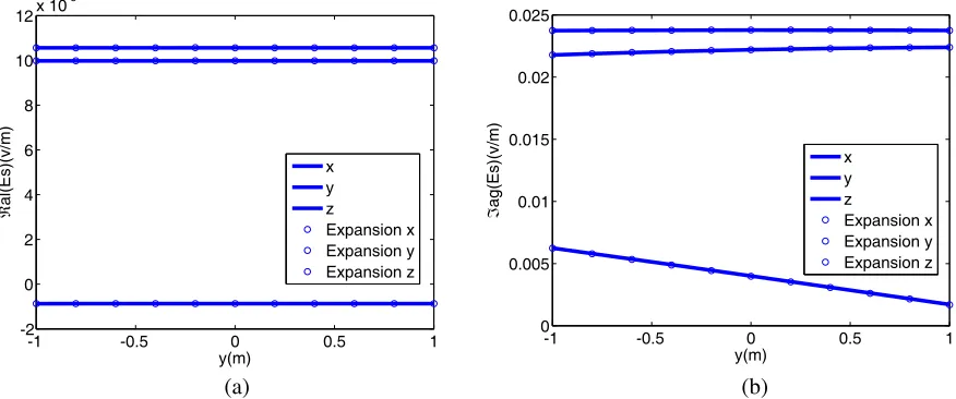
To test the accuracy of the expansion of the scattering field, the scattering solution by one RWG basis in Eq. (18) is compared with the direct method in Eq. (17). Here we randomly picked an RWG basis from one of the 435 basis for the discretization of PEC sphere located at the origin with radius of 1 m. The current coefficient on the RWG basis a_i is set as 1.0. The frequency is 0.3 MHz. The scattering field outside the PEC surface at x= 0.0 m,y ∈[−1.0, 1.0] m,z = 30.0 m which is 0.01λaway from the PEC sphere is calculated. The results are shown in Fig. 2. In this example, the vector wave function truncation numberP is chosen as 8 in Eq. (18). We can see a good agreement between the scattering fields by the expansion method and the direct method.

-1 -0.5 0 0.5 1 -2

0 2 4 6 8 10 12x 10

5

y(m)

ℜ

al(Es)(v/m)

x y z

Expansion x Expansion y Expansion z

-10 -0.5 0 0.5 1 0.005

0.01 0.015 0.02 0.025

ℑ

ag(Es)(v/m)

y(m)

x y z

Expansion x Expansion y Expansion z

(a) (b)

Figure 2. Scattered field from a RWG basis by the direct method and expansion method. (a) Real (Es). (b) Imag (Es).

5.2. Example 2: Scattering of Multiple PEC Spheres

This example is the scattering of a 2×2 sphere array. The centers of the four spheres are located at (0, 0, 0) m, (−3,0, 0) m, (0, 3, 0) m and (−3, 3, 0) m respectively. The dipole incidence is at 0.03 GHz, located at (20, 1.5, 0) m and radiates in −xˆ direction with the magnitude of 100. The radius of each sphere is 1.0 m. Each of them is discretized into 4,044 RWG basis functions. The proposed T-matrix method and CFIE with MLFMA method are used to calculate the RCS and scattered fields respectively. Fig. 3 shows the RCS results by the two methods. They have a good agreement. The near field results are shown in Fig. 4. The observation points are along a circle of 5 m around the spheres on thex-ysurface. Fig. 4(a) shows the real part of thex component of the scattered field. Fig. 4(b) shows imaginary part of the x component of the scattered field. Both of them agree well with those from the CFIE with MLFMA method.

0 20 40 60 80 100 120 140 160 180 -50

-40 -30 -20 -10 0 10 20

θ(Deg)

RCS(dB/

λ

2)

MOM T matrix

Figure 3. RCS of four PEC spheres at 0.03 GHz.

0 50 100 150 200 250 300 350 -0.5

0 0.5 1 1.5 2 2.5 3

θ(Deg)

Real(Esx)

MOM T matrix

0 50 100 150 200 250 300 350 -1.5

-1 -0.5 0 0.5 1 1.5 2

θ(Deg)

Imag(Esx)

MOM T matrix

(a) (b)

Figure 4. Scattered field of four PEC spheres at 0.03 GHz. (a) Real (E_sx). (b) Imag (E_sx).

0.04

0.02

0

0.02

0.04

0.06

0.08

0.1 0.02

0 0.02

0.04 0.06

0.08 0.02

0 0.02

Figure 5. Mesh configuration of a 2×2 antenna array.

0 20 40 60 80 100 120 140 160 180

15 20 25 30 35 40 45

θ(degrees)

RCS(dB/

λ

2)

MOM T matrix

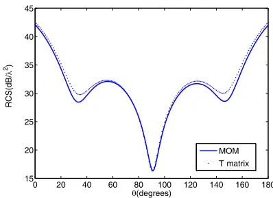
Figure 6. RCS of the 2×2 antenna array.

5.3. Example 3: Scattering of an Antenna Array

2856×4. Each of them is modelled by a T matrix. P is taken as 15. The reduction in the number of unknowns is 98.95%. Fig. 6 shows that the RCS results by the proposed method and the moment method have good agreement. As for the simulation time, the total simulation time for the EFIE with 2-level MLFMA is 30 mins, and the final matrix solving time for the T-matrix method is several seconds.

6. CONCLUSION

We developed a T-matrix method for modeling the electromagnetic scattering of multiple PEC objects. The T-matrix for a single PEC object with an arbitrary shape is derived based on the vector addition theorem combined with traditional EFIE, MFIE or CFIE method. Numerical examples for both spherical and non-spherical array structures demonstrate the accuracy and efficiency of the proposed method. The main features of the proposed method can be summarized as:

• The T-matrix for a single object only depends on its size, shape and electrical properties. It does not depend on the incidence, polarization, observation point and location of the object. Hence, it is not necessary to re-derive the T-matrix for an object when the incident field or the observation point changes or the location of the object changes. For two PEC objects with the same shape and size, they have the same T-matrix.

• By combining the vector addition theorem with the traditional EFIE, MFIE or CFIE method, the proposed method is not limited to spherical objects, it can be applied to any object with an arbitrary shape.

• The size of the T-matrix is related to the electrical size of the object. As the size of the object increases, the dimension of its T-matrix increases. However, the size of the T-matrix often much smaller than that of the corresponding MOM impedance matrix, which makes it more efficient in terms of the computational cost for the final matrix solving for multiple objects.

• One major limitation for the proposed T-matrix method is that it only works for well-separated structures, it can not apply to structures with overlaps.

ACKNOWLEDGMENT

Major part of this work is done during the author’s PhD study at University of Illinois at Urbana-Champaign under Prof. W. C. Chew’s advisement. The author would like to thank Prof. W. C. Chew for his instruction to the work.

REFERENCES

1. Waterman, P. C., “Matrix formulation of electromagnetic scattering,” Proc. IEEE, Vol. 53, 805– 812, 1965.

2. Peterson, B. and S. Strom, “T matrix for electromagnetic scattering from an arbitrary number of scatterers and representations of E(3)*,” Physical Review, Vol. 8, No. 10, 3661–3678, Nov. 1973. 3. Wang, Y. M. and W. C. Chew, “An efficient algorithm for solution of a scattering problem,”

Microwave and Optical Technology Letters, Vol. 3, No. 3, 102–106, Mar. 1990.

4. Wang, Y. M. and W. C. Chew, “A recursive T-matrix approach for solution of electromagnetic scattering by many spheres,” IEEE Trans. on Antennas and Propagation, Vol. 41, No. 12, 1633– 1639, Dec. 1993.

5. Gurel, L. and W. C. Chew, “A recursive T-matrix algorithm for strips and patches,”Radio Science, Vol. 27, No. 3, 387–401, May–Jun. 1992.

6. Chew, W. C., “Vector addition theorem and its diagonalization,”Commun. Comput. Phys., Vol. 3, No. 2, 330–341, Feb. 2008.

7. Chew, W. C.,Waves and Fields in Inhomogeneous Media, IEEE Press, 1995.

9. Mackowski, D. W. and M. I. Mishchenko, “Calculation of the T-matrix and the scattering matrix for ensembles of spheres,”J. Opt. Soc. Am. A, Vol. 13, 2266–2278, 1996.

10. Xu, H. X., “Calculation of the near field of aggregates of arbitrary spheres,” J. Opt. Soc. Am. A, Vol. 21, No. 5, 804–809, May 2004.

11. Forestiere, C., G. Iadarola, L. D. Negro, and G. Miano, “Near-field calculation based on the T-matrix method with discrete sources,”Journal of Quantitative Spectroscopy &Radiative Transfer, Vol. 112, 2384–2394, 2011.

12. Zhang, Y. J. and E. P. Li, “Fast multipole accelerated scattering matrix method for multiple scattering of a large number of cylinders,” Progress In Electromagnetics Research, Vol. 72, 105– 126, 2007.

13. Hao, S., P. G. Martinsson, and P. Young, “An efficient and highly accurate solver for multi-body acoustic scattering problems involving rotationally symmetric scatterers,” Computers &

Mathematics with Applications, Vol. 69, 304–318, 2015.

14. Kim, K. T. and B. A. Kramer, “Direct determination of the T-matrix from a MOM impedance matrix computed using the Rao-Wilton-Glisson basis function,” IEEE Trans. on Antennas and Propagation, Vol. 61, No. 10, 5324–5327, 2013.