A Fast Finite Difference Delay Modeling Solution of Transient
Scattering from Lossy Inhomogeneous Dielectric Objects
Ji Ding*, Yanfang Wang, and Jianfeng Li
Abstract—A fast finite difference delay modeling (FDDM)-based scheme is presented for analyzing transient electromagnetic scattering from lossy inhomogeneous dielectric objects. The proposed scheme is formulated in the region of the scatterers by expressing the total field as the sum of the incident field and the radiated field due to both the polarization and conduction current density. The current density is discretized in space by Schaubert-Wilton-Glisson basis functions and in time by finite differences. Furthermore, the scheme is accelerated by the fast Fourier transform (FFT) algorithm, which can reduce the memory requirement and computational complexity significantly. Numerical results are presented to illustrate the accuracy and efficiency of the proposed method.
1. INTRODUCTION
Transient electromagnetic scattering from lossy inhomogeneous dielectric objects has received considerable attention and has many applications including high-speed circuits, medical diagnostics, electromagnetic coupling and interference, etc. Among the available transient solution techniques, time domain integral equations (TDIE)-based methods are suitable to analyze electromagnetic scattering problem. One of these methods to solve TDIE is the marching-on-in-time (MOT) algorithm [1, 2]. The MOT algorithm has been widely used in the last years, but this scheme suffers from late-time instability in the form of high frequency oscillation which greatly limits its application. Recently, another alternative method, viz. the finite difference delay modeling (FDDM) algorithm [3, 4], is developed. Its temporal discretization is made based on a finite difference with a mapping from the Laplace domain to the Z-transform domain. Temporal convergence is governed by the order of the finite difference approximation. Due to the disposition of the left half plane of the Laplace domain after transformation to the Z-domain, the FDDM algorithm appears absolutely stable for any structure and any time step size.
The FDDM method has been successfully implemented for the analysis of electromagnetic scattering from perfect electric conductor objects and homogeneous dielectric objects. For perfect electric conductor objects, the FDDM method has been applied to solve the electric field integral equation (EFIE), the magnetic field integral equation (MFIE), and the combined field integral equation (CFIE) [3]. For homogeneous dielectric objects, the FDDM method has been applied to solve the Poggio-Miller-Chang-Harrington-Wu-Tsai (PMCHWT) equation [5]. In this paper, the FDDM method is extended to solve the time-domain volume integral equation (TDVIE) for the analysis of transient scattering from lossy inhomogeneous dielectric objects. The TDVIE are superior when the dielectric material is inhomogeneous or complex such as the lossy and anisotropic media [6–9]. The use of Green’s function and enforcement of the continuity condition between the normal component of the electric flux density in the dielectric body ensure a good accuracy of the solution. Despite these advantages, because VIE produces huge number of unknowns, the proposed FDDM-based scheme needs
Received 16 October 2015, Accepted 24 November 2015, Scheduled 10 December 2015
* Corresponding author: Ji Ding ([email protected]).
excessive memory requirement and computational complexity. To alleviate this problem, the FDDM-based scheme is accelerated by the fast Fourier transform (FFT) scheme [10, 11], which can reduce the memory requirement and computational complexity from O(KN2
v) and O(KNtNv2) to O(KNv) and
O(KNv(logNv + log22K)). Here, K is the truncation number, Nv is the total number of the spatial
basis functions, andNt is the number of time steps in the analysis.
The remainder of this paper is organized as follows. Section 2 describes the FDDM-based scheme to solve TDVIE and its acceleration. Section 3 gives several numerical results to demonstrate the accuracy and efficiency of the proposed method. Section 4 presents our conclusions.
2. FORMULATIONS
2.1. FDDM Solution of Volume Integral Equation
Consider an inhomogeneous lossy dielectric scatterer with a volume V residing in free space, excited by an incident electromagnetic fieldEi(r, t) that are temporally bandlimited to a maximum frequency fmax. It is assumed that frequency independent permittivity and conductivity of the scatterer are characterized by (r) and σ(r), respectively. The electromagnetic fields in the dielectric body satisfy Maxwell equation
∇ ×H(r, t) = ∂E(r, t)
∂t +J(r, t). (1)
Here, E(r, t) and H(r, t) are the total electric and magnetic fields, and the equivalent volume current densityJ(r, t) is
J(r, t) =κ(r)∂D(r, t)
∂t +ν(r)D(r, t), (2)
where D(r, t) = (r)E(r, t) is the electric flux density, κ(r) = ((r)−0)/(r), and ν(r) = σ(r)/(r). The scattered fieldEs(r, t) from the inhomogeneous scatterer can be considered as the field radiated by the equivalent volume current density J(r, t)
Es(r, t) =−μ0 4π
∂ ∂t
V
J(r, t−R/c)
R dr
+ ∇
4π0
V
t−R/c
−∞
∇·J(r, t)
R dt
dr, (3)
where R = |r−r| is the distance between the observation point r, and the source point r. c is the speed of light in free space. Since the total field is the sum of the incident field and scattered field
E(r, t) =Ei(r, t) +Es(r, t), (4) substituting Eq. (3) into Eq. (4) and differentiating Eq. (4) in time domain, the time-domain volume integral equation can be written as
∂Ei(r, t)
∂t =
1 (r)
∂D(r, t)
∂t +
μ0 4π
∂2 ∂t
V
J(r, t−R/c)
R dr
− ∇
4π0
V
∇·J(r, t−R/c)
R dr
. (5)
The finite difference delay modeling (FDDM) method works on the Laplace transform of the above equation. The Laplace transform of a function f(t) will denote byf(s). Thus, Eq. (5) transforms into
sEi(r, s) = sD(r, s)
(r) +
μ0 4π
V
sκ(r) +ν(r)D(r, s)s
2e−sR/c
R dr
− 1
4π0∇
V
∇·sκ(r) +ν(r)D(r, s)e−sR/c
R dr
. (6)
For the spatial discretization, the unknown electric flux density D(r, s) in the Laplace domain can be expanded by a set of Nv spatial basis functions
D(r, t) =
Nv
n=1
where fn(r) is thenth spatial basis function and Dn(s) the unknown expansion coefficient offn(r). In
our implementation, fn(r) are chosen to be the Schaubert-Wilton-Glisson (SWG) basis functions [12]. By expanding the electric flux density as Eq. (7) and applying a spatial Galerkin testing procedure to Eq. (6), the following matrix equation is obtained
Z(s)D(s) =V(s). (8)
Next, for the temporal discretization of Eq. (8), the Laplace variable s is replaced by with the function f(z). Eq. (8) is transformed from the Laplace domain to the Z-domain. To ensure the late-time stability, the first-order backward difference (BE) or the second-order backward difference (BDF2) is employed to approximate s=f(z) = dkz−k. The BE formula is given bys= (1−z−1)/Δt and the
BDF2 formula is given by s= (3−4z−1+z−2)/(2Δt). Thus, the terms sle−sR/c are expanded by the Laurent series as
sle−sR/c|s=f(z)=
K
k=0
w(kl)z−k, (9)
wherew(kl) is the expansion coefficients. Since w(kl) converge rapidly, we can truncate the summation at some finite numberK. The expansion coefficients for the BE formula are given by
wk(0) = 1
k!
R cΔt
k/2
e−R/cΔt, (10)
w(kl) = 1 Δt
wk(l−1)−wk(l−−11)
, (11)
and the expansion coefficients for the BDF2 formula are given by
wk(0) = 1
k!
R 2cΔt
k/2
Hk
2R cΔt
e−3R/2cΔt, (12)
w(kl) = 1 2Δt
3w(kl−1)−4w(kl−−11)+w (l−1)
k−2
, (13)
where Hk(·) is the kth-order Hermite polynomial. By taking inverse Z-transform of Eq. (9), the
multiplication in theZ-domain becomes a convolution in the time domain, the following matrix equation is obtained
Z0Dj =Vj− K
k=1
ZkDj−k, (14)
for 0≤j≤Nt, whereNtis the number of the time steps. Dj is the unknown current vector andVj the
voltage vector atjth time step, respectively. Assuming that the currents up to the (j−1)th time step are known, this equation permits the computation of the currents associated with the jth time step. Therefore, the currents at all time steps can be computed recursively. The elements of the matrix Zk
can be computed as
Zk(m, n) =dk
Vm
fm(r)·
fn(r)
(r) dr+Z
κ
k(m, n) +Zνk(m, n), (15)
where
Zκk(m, n) =
Vm
Vn
μ0wk(3)
4π fm(r)·κ(r )f
n(r)
+w (1)
k
4π0
[∇ ·fm(r)−nˆ·fm(r)][∇·κ(r)fn(r)]
1 Rdr
dr, (16)
Zνk(m, n) =
Vm
Vn
μ0w
(2)
k
4π fm(r)·ν(r )f
n(r)
+w (0)
k
4π0
[∇ ·fm(r)−nˆ·fm(r)][∇·ν(r)fn(r)]
1 Rdr
In Eq. (14), the computational bottleneck is the matrix-vector multiplication of the right-hand side. The memory requirement and computational complexity of the FDDM-based scheme areO(KN2
v) and
O(KNtNv2). Such memory requirement and computational complexity are highly excessive. In the next
section, the FFT scheme will be employed to alleviate this problem.
2.2. FFT Acceleration
To implement the FFT scheme to accelerate the matrix-vector multiplications of Eq. (14), the entire scatterer must be enclosed within an auxiliary 3-D Cartesian grid with Nc = Nx ×Ny ×Nz
nodes. Assume the spacings of the auxiliary grid Δs are identical. The spatial basis functions {fm(r), χ(r)fn(r),∇ ·fm(r)−nˆ·fm(r),∇ ·χ(r)fn(r)} (χ=κ, ν) are locally projected onto the auxiliary grid and can be approximated as a linear combination of Dirac delta functions
fm(r) =
(M+1)3
u=1
[Γxmuxˆ+ Γymuˆy+ Γzmuˆz]δ(r−ru)
χ(r)fn(r) = (M+1)3
u=1
[Λχxnuxˆ+ Λχynuyˆ+ Λχznuˆz]δ(r−ru)
∇ ·fm(r)−nˆ·fm(r) =
(M+1)3
u=1
Γdmuδ(r−ru)
∇ ·χ(r)fn(r) =
(M+1)3
u=1
Λχdnuδ(r−ru). (18)
whereM is the expansion order, andru represents nodeuon the auxiliary grid. Γx,y,z,dmu and Λχx,χy,χz,χdnu
are the expansion coefficients which can be determined by using the multipole expansion [13]. When the observation points are beyond a nominal distance from the primary source, the auxiliary basis function can reproduce the equivalent transient fields of the primary source with high accuracy.
Once the spatial basis functions are projected onto the auxiliary grid, substituting Eq. (18) into Eqs. (16) and (17), the matrix elements of Zk can be approximated by replacing the primary basis functions with the auxiliary basis functions
Zκk(m, n) =
(M+1)3
u=1
(M+1)3
v=1
μ0w (3)
k
4πR [Γ
x
muxˆ+ ΓymuyΓˆ zmuˆz]·[Λκxnvxˆ+ Λκynvyˆ+ Λκznvˆz] +
w(1)k 4π0R
ΓdmuΛκdnv, (19)
Zνk(m, n) =
(M+1)3
u=1
(M+1)3
v=1
μ0w(2)k 4πR [Γ
x
muxˆ+ ΓymuyΓˆ zmuˆz]·[Λνxnvxˆ+ Λνynvyˆ+ Λνznvˆz] +
wk(0) 4π0R
ΓdmuΛνdnv, (20)
Here,R=|ru−rv|is the distance between node uand nodev. Thus, the far-field impedance matrices
Zf ark can be expressed as
Zf ark =Γ†x Γ†y Γ†z
⎛ ⎜ ⎝ ⎡ ⎢ ⎣
G(3)k Λκx G(3)k Λκy G(3)k Λκz
⎤ ⎥
⎦+
⎡ ⎢ ⎣
G(2)k Λνx G(2)k Λνy G(2)k Λνz
⎤ ⎥ ⎦
⎞ ⎟
⎠+Γ†d
G(1)k Λκd+G(0)k Λνd
, (21)
where † is the transpose of the matrix; Γx,y,z,d, Λκx,y,z,d and Λνx,y,z,d represent the sparse projection
matrices of dimensionNc×Nv, which contain (M+ 1)3 non-zero expansion coefficients in each column.
G(0)k ,(1),(2),(3) are the 3D-Toeplitz matrices of dimension Nc ×Nc whose elements are the free-space
Green’s function evaluated on the auxiliary grid
G(0)k (u, v),G(1)k (u, v),G(2)k (u, v),G(3)k (u, v) =
wk(0) 4π0R,
wk(1) 4π0R,
μ0w(2)k 4πR ,
μ0w(3)k 4πR
For the simplicity of discussion, we useΓpGpkΛp (p= 1,· · · ,8) to correspond to the eight matrix-vector multiplications in Eq. (21). Since the 3D-Toeplitz nature enables the use of 3D-FFT to compute the matrix-vector multiplication efficiently, the far-field interactions are expressed as the following unified form
Zf ark Dj−k=
8
p=1
ΓpGpkΛpDj−k=
8
p=1
ΓpF−1!F{Gkp} •F{ΛpDj−k}
"
, (23)
where F(·) and F−1(·) are the forward FFT and the inverse FFT, respectively. The dot represents element-by-element multiplication.
For the far-field interactions, Zf ark can provide good approximation. However, for the near-field interaction, Zf ark can not provide good approximation. The near-field impedance elements have to be calculated directly through Eq. (15), and the erroneous contributions from Zf ark needs to be removed from the near-field interactions. Thus, the near-field impedance matrix is defined as
Zneark (m, n) =
0, dmn> dnear
Zk(m, n)−Zf ark (m, n), dmn≤dnear,
(24)
wheredmn is the distance between the basis functionm and n, anddnear is the near-field threshold.
Substituting Eqs. (23) and (24) into Eq. (14), Eq. (14) can be represented as
Z0Dj =Vj − K
k=1
Zneark Dj−k− 8
p=1 ΓpF−1
K
k=1
F{Gpk} •F{ΛpDj−k}
=Vj −
K
k=1
Zneark Dj−k− 8
p=1 ΓpF−1
#
Vpj . (25)
Here, the forward FFTs of the sequences Gpk are pre-computed and stored before the simulation. The forward FFTs of the vectors ΛpDj−k are computed and stored during the time-marching. For 1 ≤ p ≤8, one forward FFT of ΛpDj−1, one inverse FFT, and K element-by-element multiplication operations are required per time step. These FFTs require O(NclogNc) operations per time step; the
multiplication of the two FFT sequences can take advantage of the temporal Toeplitz nature, which costsO(Nclog22K) operations per time step. Like the frequency-domain FFT-based algorithms [14, 15],
Nc is proportional to Nv. Hence, the total memory requirement and computational complexity are
O(KNv) andO(NtNv(logNv+ log22K)), respectively. It should be noted that since all the elements are real value, two real FFTs can be most efficiently performed using one complex FFT. In the practical implementation, for the sequencesGpk, only the forward FFT ofG(0)k needs to be stored, because the sum of the element-by-element multiplication of G(kl) can be evaluated recursively from the computations of G(kl−1) during the time-marching. For the BE formula, the sum of the element-by-element multiplication can be represented as
K
k=1
F{G(kl)} •F{ΛpDj−k}= 1 Δt
K
k=1
FG(kl−1)−G(kl−−11) •F{ΛpDj−k}
= 1 Δt
$ #
V(jl−1)−
#
V(jl−−11)+F{G(0l−1)} •F{ΛpDj−1} −F{G(Kl−1)} •F{ΛpDj−1−K}
%
, (26)
and for the BDF2 formula, the sum of the element-by-element multiplication can be represented as
K
k=1
F{G(kl)} •F{ΛpDj−k}= 1 2Δt
K
k=1
F3G(kl−1)−4G(kl−−11)+G(kl−−21) •F{ΛpDj−k}
= 1
2Δt $
3V#(jl−1)−4
& #
V(jl−−11)+F{G(0l−1)} •F{ΛpDj−1} −F{G(Kl−1)} •F{ΛpDj−1−K}
+
& #
Vj(l−−21)+F{G0(l−1)} •F{ΛpDj−2} −
K
k=K−1
F{G(kl−1)} •F{ΛpDj−2−k}
'%
. (27)
3. NUMERICAL RESULTS
This section presents numerical results that serve both to validate the above described scheme and to demonstrate the accuracy and efficiency. All the simulations are performed on a shared memory workstation equipped with Intel Xeon CPU E5-2603 1.8 GHz (using 4 processors in the OpenMP parallelization) and 64 GB of RAM. The expansion order isM = 3, the truncation number isK = 120, the auxiliary grid spacing is Δs= 0.08λmin, and the near-field threshold isdnear = 0.4λmin. The incident wave is a modulated Gaussian plane wave parameterized as
Ei(r, t) = ˆpexp
&
− 1
2σ2(τ−8σ) 2
'
cos(2πf0τ). (28)
Here,f0is the center frequency,τ =t−r·kˆ/c, andσ= 6/(2πfbw). fbwis the bandwidth of the incident
wave. ˆk and ˆpdenote the travel direction and polarization direction of the incident wave.
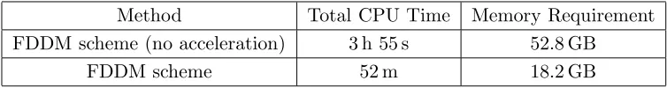
Table 1. Comparison of the total CPU time and memory requirement.
Method Total CPU Time Memory Requirement
FDDM scheme (no acceleration) 3 h 55 s 52.8 GB
FDDM scheme 52 m 18.2 GB
In the first example, we consider a dielectric half-spherical shell. The inner and outer shell radius is 0.95 m and 1.0 m, respectively. The permittivity are1(r) = 20 and2(r) = 1.50, and the conductivity are σ1(r) = 0.0055 s/m and σ2(r) = 0.0067 s/m. The incident pulse travels in ˆk=−zˆ direction and is polarized along ˆp =−x. The center frequency and bandwidth areˆ f0 = 200 MHz andfbw = 100 MHz.
The shell is discretized in terms of 10507 SWG basis functions. The time step size is Δt= 1/(20fmax), and the number of time steps is Nt = 2000. The electric flux density for ˆx direction observed at the
point (0.0 m, 0.0 m, 1.0 m) computed using the BDF2 FDDM schemes are compared with those obtained by the inverse discrete Fourier transform (IDFT) of the frequency-domain method-of-moments (MoM) solution in Fig. 1. The back-scattered far-field signal for ˆxdirection are compared in Fig. 2. The results are in good agreement with each other. Table 1 exhibits the memory requirement and total CPU time of the FDDM schemes. It can been seen that the FDDM scheme saves about 3 times memory and 4 times CPU time than that not accelerated by FFTs. With the size of the scatterer increasing, the FDDM scheme will save further more CPU time and memory requirement.
Next, transient scattering from a homogenous dielectric almond with length of 2.52374 m is analyzed. The permittivity is (r) = 20 and the conductivity is σ(r) = 0.0055 s/m. The incident pulse travels in ˆk =−ˆz and is polarized along ˆp =−x, has a center frequency ofˆ f0 = 200 MHz and bandwidth of fbw = 100 MHz. The almond is discretized using 12918 SWG basis functions. The time
step size is Δt= 1/(20fmax), and the number of time steps is Nt= 2000. The electric flux density for ˆx
direction at the point (−0.774 m,−0.135 m,−1.948 m) and the transient back-scattered far-field signal computed using the BE and BDF2 FDDM schemes are shown in Fig. 3 and Fig. 4. The results also agree well with those obtained by the IDFT of MoM solution.
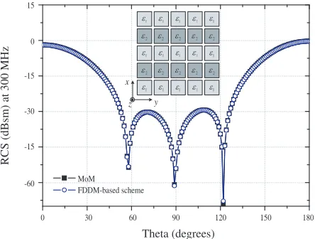
Finally, transient scattering from 5-by-5 array of dielectric cubes is analyzed. The side length of each cube is 0.15 m, and the distance between the centers of two adjacent cubes is 0.25 m. The permittivity are1(r) = 20 and 2(r) = 30, and the conductivity are σ1(r) = 0.0055 s/m andσ2(r) = 0.00255 s/m. The incident pulse travels in ˆk = −ˆz direction and is polarized along ˆp = −x. The center frequencyˆ and bandwidth aref0 = 400 MHz andfbw= 200 MHz. The array of dielectric cubes is discretized using
24808 SWG basis functions. The time step size is Δt = 1/(20fmax), and the number of time steps is
ε ε
Dx (A/m)
Time (ns) MoM
FDDM-based scheme
FDDM-based scheme (no acceleration)
1.5 × 10⁻¹¹
1.0 × 10⁻¹¹
5.0 × 10⁻¹²
0.0
-5.0 × 10⁻¹²
-1.0 × 10⁻¹¹
-1.5 × 10⁻¹¹
0 50 100 150 250 300
x y z
1 2
Figure 1. The electric flux density for ˆxdirection at (0.0 m, 0.0 m, 1.0 m) in a half-spherical shell.
ε ε
rEx (V/m)
Time (ns) MoM
FDDM-based scheme
FDDM-based scheme (no acceleration)
8.0 × 10⁻²
6.0 × 10⁻²
4.0 × 10⁻²
0.0
-2.0 × 10⁻²
-6.0 × 10⁻²
-8.0 × 10⁻²
0 50 100 150 250 300
2.0 × 10⁻²
-4.0 × 10⁻²
x y z
1 2
Figure 2. Transient back-scattered far-field response scattered by a half-spherical shell.
Dx (A/m)
Time (ns) 0.0
0 50 100 150 250 300
2.0 × 10⁻¹¹
1.0 × 10⁻¹¹
-2.0 × 10⁻¹¹
-1.0 × 10⁻¹¹
MoM
FDDM-based scheme (BE) FDDM-based scheme (BDF2)
x
y z
kinc
Figure 3. The electric flux density for ˆxdirection at the point (−0.774 m,−0.135 m,−1.948 m) in a dielectric almond.
rEx (V/m)
Time (ns) 0.2
0 50 100 150 250 300
0.6 0.4 -0.2 0.0 -0.4 -0.6 MoM
FDDM-based scheme (BE) FDDM-based scheme (BDF2)
x
y z
kinc
Figure 4. Transient back-scattered far-field response scattered by a dielectric almond.
ε ε ε ε ε
ε ε ε ε ε
ε ε ε ε ε
ε ε ε ε ε
ε ε ε ε ε
RCS (dBsm) at 300 MHz
Theta (degrees)
-30
0 30 60 90 120 150
15 0 -60 -15 -15 180 MoM FDDM-based scheme x y z
Figure 5. Comparison of the bistatic RCS obtained from the FDDM scheme and MoM for a 5-by-5 array at 300 MHz.
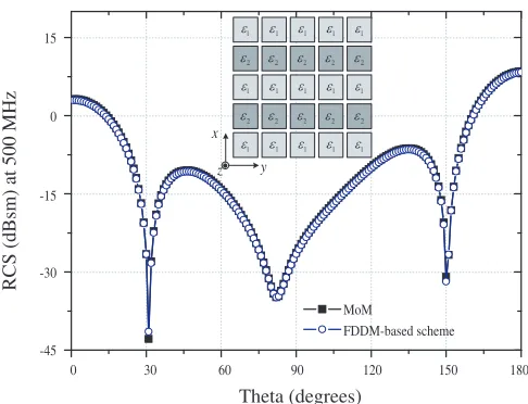
ε ε ε ε ε
ε ε ε ε ε
ε ε ε ε ε
ε ε ε ε ε
ε ε ε ε ε
RCS (dBsm) at 400 MHz
Theta (degrees)
-30
0 30 60 90 120 150
15 0 -45 -15 180 MoM FDDM-based scheme x y z
ε ε ε ε ε
ε ε ε ε ε
ε ε ε ε ε
ε ε ε ε ε
ε ε ε ε ε
RCS (dBsm) at 500 MHz
Theta (degrees) -30
0 30 60 90 120 150
15
0
-45 -15
180
x
y z
MoM
FDDM-based scheme
Figure 7. Comparison of the bistatic RCS obtained from the FDDM scheme and MoM for a 5-by-5 array at 500 MHz.
bistatic RCS was computed for φ = 0◦, and θ between 0◦ and 360◦. The RCS patterns at 300 MHz, 400 MHz, and 500 MHz obtained by the BDF2 FDDM scheme and MoM agree well with each other as shown in Figs. 5–7.
4. CONCLUSIONS
In this paper, a fast finite difference delay modeling (FDDM)-based scheme for computing transient electromagnetic scattering from lossy inhomogeneous dielectric objects is presented. This scheme is formulated in the region of the scatterers by expressing the total fields as the sum of the incident field and the radiated field due to both the polarization and conduction current density. The temporal discretization based on first- and second-order backward difference makes the scheme absolutely stable. Additionally, the memory requirement and computational complexity have been reduced remarkably by using the fast Fourier transform algorithm. Numerical results about electromagnetic scattering from lossy inhomogeneous dielectric objects are presented to illustrate the accuracy and efficiency of our method. In our future work, the FDDM-based scheme will be developed to analyze transient scattering from dispersive dielectric objects using integral equation.
ACKNOWLEDGMENT
This paper is supported by the Postdoctoral Science Foundation of China (Grant No. 2015M571654), NSF-China and Guangdong Province Joint Project (Grant No. U1301252 ), and National Natural Science Foundation of China (Grant No. 61272543).
REFERENCES
1. Rao, S. M. and D. R. Wilton, “Transient scattering by conducting surfaces of arbitrary shape,” IEEE Trans. Antennas Propagat., Vol. 39, No. 1, 56–61, 1991.
2. Shanker, B., A. A. Ergin, K. Aygun, and E. Michielssen, “Analysis of transient electromagnetic scattering from closed surfaces using a combined field integral equation,” IEEE Trans. Antennas Propagat., Vol. 48, No. 7, 1064–1074, 2000.
4. Wang, X. B. and D. S. Weile, “Implicit Runge-Kutta methods for the discretization of time domain integral equations,” IEEE Trans. Antennas Propagat., Vol. 59, No. 12, 4651–4663, 2011.
5. Wang, X. B. and D. S. Weile, “Electromagnetic scattering from dispersive dielectric scatterers using the finite difference delay modeling method,” IEEE Trans. Antennas Propagat., Vol. 58, No. 5, 1720–1730, 2010.
6. Gres, N., A. A. Ergin, B. Shanker, and E. Michielssen, “Volume integral equation based analysis of transient electromagnetic scattering from three-dimensional inhomogeneous dielectric objects,” Radio Sci., Vol. 36, 379–386, 2001.
7. Shanker, B., K. Aygun, and E. Michielssen, “Fast analysis of transient scattering from lossy inhomogeneous dielectric bodies,”Radio Sci., Vol. 41, 39–52, 2004.
8. Kobidze, G., J. Gao, B. Shanker, and E. Michielssen, “A fast time domain integral equation based scheme for analyzing scattering from dispersive objects,”IEEE Trans. Antennas Propagat., Vol. 53, No. 3, 1215–1226, 2005.
9. Jung, B.-H., Z. Mei, and T. K. Sarkar, “Transient wave propagation in a general dispersive media using the Laguerre functions in a marching-on-in-degree (MOD) methodology,” Progress In Electromagnetics Research, Vol. 118, 135–149, 2011.
10. Yilmaz, A. E., D. S. Weile, J. M. Jin, and E. Michielssen, “A hierarchical FFT algorithm (HIL-FFT) for the fast analysis of transient electromagnetic scattering phenomena,” IEEE Trans. Antennas Propagat., Vol. 50, No. 10, 971–982, 2002.
11. Yilmaz, A. E., J. M. Jin, and E. Michielssen, “A fast Fourier transform accelerated marching-on-in-time algorithm for electromagnetic analysis,” Electromagnetics, Vol. 21, 181–197, 2001.
12. Schaubert, D. H., D. R. Wilton, and A. W. Glisson, “A tetrahedral modeling method for electromagnetic scattering by arbitrarily shaped inhomogeneous dielectric bodies,” IEEE Trans. Antennas Propagat., Vol. 32, No. 1, 77–85, 1984.
13. Bleszynski, E., M. Bleszynski, and T. Jaroszewicz, “AIM: Adaptive integral method for solving large-scale electromagnetic scattering and radiation problems,” Radio Sci., Vol. 31, 1225–1251, 1996.
14. Zhang, Z. Q and Q. H. Liu, “A volume adaptive integral method (VAIM) for 3-D inhomogeneous objects,” IEEE Antennas Wireless Propag. Lett., Vol. 1, 102–105, 2002.