A Steerable Least Square Approach for Pattern Synthesis

A Steerable Least Square Approach for Pattern Synthesis

Jie Chen1, *, Yingzeng Yin2, and Yongchang Jiao2

Abstract—The least square method has been widely applied in many fields. However, when the approach is used for antenna array pattern synthesis, it is not excellent. In this paper, the least square method is used to synthesize antenna array pattern, and its performance is reviewed. Then contraposing to the shortcoming of the least square method, a new steerable least square (SLS) method is put forward. For an antenna array whose manifold matrix has been determined, the projection matrix equation can be derived from array manifold matrix easily. In order to get premium solution of array element excitation, a novel projection matrix equation with adjustable matrices is adopted. The results of simulations show that the pattern synthesized by the traditional least square method fits the targeted pattern badly and is worse in the key performance indicators of peak level of side-lobe and null beam level than the targeted pattern; however, the pattern synthesized by the new SLS method fits the targeted pattern well in zero point and local peak distribution and is better in the key performance indicators of peak level of side-lobe and null beam level than the targeted pattern.

1. INTRODUCTION

Beam forming and antenna array pattern synthesis technology have been well investigated in the past fifty years. Application of beam forming in commercial wireless communication sector has become wider and wider in recent years. It has been put into use in the systems of input multiple-output (MIMO) radar and smart antenna. In early time, beam forming was accomplished in radio frequency front end where phase shifters and radio amplifiers were used to weight the antenna element excitation. This structure is sizable, cumbersome and short of flexibility. Microwave beam forming (MBF) is an attractive alternative. In this structure, a digital to analog converter (DAC) branch and one radio frequency conversion unit are used, and only one signal is transferred to the transmitting radio frequency front end. Several techniques have been developed to implement adaptive beam forming (ABF) on the MBF structure system [1, 2]. Digital beam forming (DBF) is another hot technology that allows using digital signal processing operations on the antenna array signals. Beam formed by digital signal processing can be flexibly changed and conveniently upgraded.

To date, many beam forming and pattern synthesis approaches have been developed by researchers [4–19]. The first approach in which the transmitting pattern design in general is investigated is well-known analytic function method, such as Chebyshev and Taylor pattern synthesis. In the second method, beam forming is considered as a spatial filtering issue [3]. Researchers view beam forming as a nonlinear optimization issue and use numerical means to get the antenna element excitation or weighting vector in the third type approach. Aside from these, many researches are devoted to developing fast computing algorithms to adapt to real time processing of beam forming and null forming [4, 5].

Recently, for the purposes of reducing processing time and improving calculating speed, many articles have been published. In [6], authors discuss a beam forming approach used in wide-band MIMO

Received 24 May 2017, Accepted 4 August 2017, Scheduled 18 August 2017 * Corresponding author: Jie Chen (chenbinglin88888@163.com).

system. A compressed sensing method is applied to form beam in [7]. The authors of [8] investigate beam forming method under the limitation of l1-norm minimization. In [9], a real weight adaptive processing based on direct data domain least square approach is proposed to implement real time beam forming. In [10], the least square method has been universally applied in signal processing and beam forming. In [11–19], various methods for pattern synthesis are presented.

The least square method has been widely applied in many fields. However, when the approach is used for antenna pattern synthesis, it is not excellent. Actually, in many occasions, the pattern synthesis outcomes of the least square method are not satisfactory.

In this paper, the least square method is used to synthesize antenna array pattern, and its performance is reviewed. Then contraposing to the shortcoming of the least square method, a new steerable least square (SLS) method is put forward. For an antenna array whose manifold matrix has been determined, the projection matrix equation can be derived from array manifold matrix easily. In order to get premium solution of array element excitation, a novel projection matrix equation with adjustable matrices is adopted. The results of simulations show that the pattern synthesized by the traditional least square method fits the targeted pattern badly and is worse in the key performance indicators of peak level of side-lobe and null beam level than the targeted pattern; however, the pattern synthesized by the new SLS method fits the targeted pattern well in zero point and local peak distribution, and is better in the key performance indicators of peak level of side-lobe and null beam level than the targeted pattern.

The new SLS method reforms the traditional least square projection matrix equation into a new matrix equation with variable parameters, which overcomes the shortcoming of the least square method. The new method can get premium solution of the array pattern synthesis, and it has never been found before.

The rest parts of this paper are organized as follows. In Section 2, the pattern synthesis paradigm is given. The new steerable least square (SLS) method for pattern synthesis is presented in Section 3. Simulation examples are shown in Section 4. In Section 5, several attributes of the new approach are discussed, including application for other array geometries and other application fields, mutual coupling effects, computation complexity and performance. In Section 6, the conclusion is drawn.

2. PATTERN SYNTHESIS PARADIGM

A d-spaced uniform linear antenna array withN isotropic elements is taken as the object of the study. The scenario in far field is considered while narrow band beam with the central wave length λ is transmitted by all antenna elements. As shown in Figure 1, the antenna elements distribute along a line with the number from 0 to N −1. The signal angle, or the signal transmitting angle, is the angle between signal and the axis of array denoted asθ.

.

..

θ

... i i+1 ...

...

As shown in Figure 1, pattern formed in far field is

f(θ)=

N−1

i=0

Iiej2πidcosθ/λ (1)

In Equation (1), Ii is theith antenna element’s current excitation.

Equation (1) can be rewritten as

f(θ)=aT(θ)W (2)

Given the fact that the pattern is the periodic function of cosθ, we consider only the case whereθ is in the scope from 0◦ to 180◦. For the convenience of digital processing, we denote the discrete value ofθ

asθ1, θ2, . . . , θk, . . . , θK in turn, where kis an integer. Let the targeted pattern vector be

P= [P(θ1), P(θ2), . . . , P(θk), . . . , P(θK)]T = [P1, P2, . . . , Pk, . . . , PK]T (3)

So, the problem of pattern synthesis is to obtain the weighting vector W by solving the equation

abs

[a(θ1),a(θ2), . . . ,a(θk), . . . ,a(θK)]T W

=P (4)

In Equation (4), abs denotes absolute value operation. Let

A= [a(θ1),a(θ2), . . . ,a(θk), . . . ,a(θK)] (5)

called as array manifold matrix.

So, Equation (4) can be rewritten as

absATW=P (6)

There are many strategies to solve Equation (6). The simplest and most usual way is to transform Equation (6) into

ATW=P (7)

or

minATW−P2 (8)

where · denotes vector length.

After absolute value operation in Equation (6) is removed, the solving processes of Equations (7) and (8) are simplified. There are many traditional methods to solve Equations (7) and (8). The most common method is the least square method [10]. The least square solution of Equation (7) or (8) is

W_LS =ATHAT−1ATHP (9)

where superscriptH indicates conjugate transpose operation.

3. THE NEW STEERABLE LEAST SQUARE METHOD FOR PATTERN SYNTHESIS

In practice, the pattern synthesized by the least square solution cannot fit the expected pattern well. It is necessary to ameliorate this method to get a better outcome.

LetG=AT_{, and Equation (7) can be rewritten as}

GW=P (10)

The least square solution of Equation (9) can be rewritten as

WLS =

GHG−1GHP (11)

Let

D= diag(P) =diag [P1, P2, . . . , PK] (12)

In this equation, diag denotes diagonal matrix. From Equation (10), we can get

(D)−1GW= (D)−1P=E (13)

whereE is a column vector with all elements being 1. Then, the following equation can be gotten

So,

W =

GH(D)−1G

₋1

GHE (15)

On the other hand, because

P=DE, (16)

from Equation (11) we can get

W =GHG−1GHDE (17)

It is obvious that Equations (15), (17) and (11) all are solutions of Equation (10). Comparing Equations (15) and (17) with (11), because E is a column vector whose all elements are 1, we can conclude that D in both Equations (15) and (17) play the same role asPin Equation (11).

Let

P1l+m+1,P2l+m+1, . . . ,Pkl+m+1, . . . ,PKl+m+1

T _define

= Pl+m+1 (18)

where bothl andm are integer variables.

When being measured in the unit of dB, patternPis 10lgP, andPl+m+1is (l+m+ 1)10lgPwith lg denoting common logarithm operation. It is obvious thatPl+m+1has better directivity and bigger gain thanP. Based on this knowledge, in order to enhance directivity of the array, the following equation is considered.

GW=Pl+m+1 (19)

If Wsatisfies Equation (19), the pattern formed byW will have better directivity and bigger gain than P.

As the same principle mentioned previously, from Equation (19) we can get

D−1lGW=D−1lPl+m+1=Pm+1 = (D)mP. (20)

So

GHD−1lGW=GH(D)mP (21)

Then, we can get

W=

GHD−1lG

₋1

GH(D)mP (22)

It is easy to obtain other expressions which are

W=

GHD−1lG

₋1

GH(D)m+1E (23)

and

W =

GHD−1l+m+1G

₋1

GHE (24)

and

W=

GHD−1l+mG

₋1

GHP (25)

and

W=GHG−1GHPl+m+1. (26)

4. THE SIMULATIONS OF THE NEW APPROACH

Several examples are taken to exhibit the new approach and its performance in this section.

As shown in Figure 1, we consider the case in far field. Letd=λ/2. Given the fact that the beam pattern is a periodic function of the signal transmitting angle θ, we set θ in a period scope from 0◦ to 180◦. Let its discrete value θ1, θ2, . . . , θk, . . . , θK equal to 0◦,1◦, . . . ,179◦,180◦ in turn. These settings are consistent with the real practice and are convenient for digital processing.

In the first example, letN = 25, and the targeted pattern P0 is generated by uniform amplitude excitation and can be written as

P0(θ) =

N−1

i=0

Iej2πid(cosθ−cosθ0)/λ

(27)

in which θ is the signal transmitting angle as shown in Figure 1, θ = π/2 the scan angle, and I the amplitude of current excitation. From Equation (22), we obtain the element excitation vectorW of the synthesized pattern. Then the formed pattern can be obtained from Equation (7).

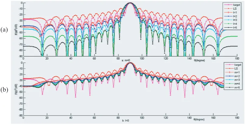
Let D = diag(P0), and the simulation outcomes are shown in Figure 2. Figures 2(a) and 2(b) indicate the cases of m = 0 and l = 0, respectively. In the column of the legend of Figure 2, target denotes expected pattern created by Equation (27); LS refers to pattern formed by the traditional least square solution of Equation (9); l = 1, l = 2, l = 3, l = 4, l = 5 and m = 1, m = 2, m = 3, m = 4,

m= 5 are the patterns created by the element excitation of Equation (22) whilemand lhave different values.

(a)

(b)

Figure 2. The outcomes of simulation (N = 25); In the column of legend, target denotes the expected beam pattern created by Equation (27), LS refers to the pattern formed by the traditional least square solution of Equation (9), l= 1, l= 2, l= 3, l= 4, l= 5 and m= 1, m= 2, m = 3, m= 4, m= 5 are the patterns created by the element excitation of Equation (22) while D = diag(P0). Figures (a) and (b) indicate the case ofm= 0 and l= 0 respectively.

In Figure 2(a), when m = 0, the main-lobe of the targeted pattern is in the range from 85◦ to 95◦, and its first side-lobe peak level is −13.8 dB. The main-lobe of the least square method is in the range from 84◦ to 96◦, and its first side-lobe peak level is−9.8 dB. The main-lobes of the new approach expand increasingly from [84◦ 96◦] to [81◦ 99◦] while l increases from 1 to 5. The first side-lobe peak levels are −16.3 dB while l = 1; −25.9 dB while l = 2; −30.0 dB while l = 3; −29.6 dB while l = 4;

−28.9 dB whilel= 5. It is noticeable that whilelincreases from 3 to 5, the levels slump as the pace of

In Figure 2(b), both the targeted and least square’s patterns are the same as that in Figure 2(a). Whenmchanges from 1 to 5 withl= 0, the first side-lobe peak levels are−12.5 dB,−13.0 dB,−13.4 dB,

−13.7 dB, −13.9 dB, respectively. A fact needed to point out is that in the case of l = 0 as shown in Figure 2(b) Equation (26) becomes

W=GHG−1GHPm+1 (28)

Actually, this is the traditional least square solution while the targeted pattern is Pm+1.

From Figure 2, we can learn that for all the cases under the condition of l= 0, all the zero point levels are much higher than those of target pattern. However, for all the cases under the condition of

m = 0, the zero point distribution along the angle variable θ is nearly the same as that of the target pattern, and all the zero point levels are lower than those of target pattern. From these data, it is apparent that parameterl has more effects on outcomes than m.

In the second example, still letN = 25, and all conditions are the same as those in the first example except that there is a null beam with the minimum level of−87 dB in expected pattern whenθis within the interval [127◦, 133◦]. The null beam is generated by programme. The simulation results are shown in Figure 3.

(a)

(b)

Figure 3. The outcomes of simulation (N = 25); In the column of legend, target denotes expected beam pattern, LS refers to pattern formed by the traditional least square solution of Equation (9),

l = 1, l = 2, l = 3, l = 4, l = 5 andm = 1, m = 2, m = 3, m = 4, m = 5 are the patterns created by the element excitation of Equation (22). Figures (a) and (b) indicate the case of m = 0 and l= 0 respectively.

In Figure 3(b), both the targeted and least square’s patterns are almost the same as those in Figure 3(a). When m changes from 1 to 5 with l = 0, the new method has nearly the same results as those in Figure 2(b). There is still no null beam in the patterns whilemchanges from 1 to 5 withl= 0. This shows that in Equation (22) parameterl has more effects on outcomes than m.

In the third example, still let N = 25, and all conditions are the same as those in the second example. This example simulates the case ofl= 1,m= 1;l= 2,m= 2;l= 3,m= 3;l= 4,m= 4 and

l= 5, m = 5. As pointed out in Figure 4, the traditional least square, indicated by LS, is a degraded form of Equation (22) whilel= 0,m= 0 actually.

Figure 4. The outcomes of simulation (N = 25); In the column of legend, target denotes the expected beam pattern, LS refers to the pattern formed by the traditional least square solution of Equation (9),

l= 1, m= 1;l= 2, m= 2; l= 3, m= 3; l= 4, m= 4 andl= 5,m= 5 mark the patterns created by the element excitation of Equation (22).

The simulation outcomes are shown in Figure 4. All data of these patterns approximate to those of Figure 3(a). The pattern’s first side-lobe peak level while l= 1 andm= 1 is 0.4 dB lower than that while l= 1 and m= 0 in Figure 3(a). The pattern’s first side-lobe peak levels whilel= 2 m= 2,l= 3

m= 3, l= 4 m= 4, l= 5m= 5 are 0.6 dB, 0.8 dB, 0.9 dB 0.9 dB lower than those while l= 2m= 0,

l= 3 m= 0, l= 4 m= 0, l= 5 m= 0 in Figure 3(a) in sequence. The pattern’s null beam minimum levels whilel= 1 m= 1, l= 2 m= 2,l= 3 m= 3,l= 4m= 4, l= 5m= 5 are 2.8 dB, 2.0 dB, 1.8 dB 1.3 dB, 1.1 dB lower than those whilel= 1 m= 0, l= 2m= 0, l= 3 m= 0, l= 4 m= 0,l= 5 m= 0 in Figure 3(a) in turn. It can be concluded from Figure 4 that in Equation (22) parameter l has more effects on outcomes thanm once again.

In the last example, we consider a nonuniform linear array. All antenna elements are arranged along a line same as that shown in Figure 1. Elements 0 to 8 are equally spaced by a distance d1, elements 8 to 17 equally spaced by a distance d2, and elements 18 to 24 equally spaced by a distance

d3. Let d1 =λ/3,d2 = 2λ/5, and d3 =λ/2. Pattern P1 is generated by uniform amplitude excitation and can be written as

P1(θ) =

N−1

i=0

Iej2πxi(cosθ−cosθ0)/λ

(29)

In Figure 5, the main-lobe of the target pattern is in the range from 84◦ to 96◦. The main-lobes of the traditional least square method and the cases of m = 1, m = 2, m = 3 while l = 0 all are in the same range as that of the target pattern. With m = 0, when l = 1, l = 2, l = 3 and l = 4, the main-lobes almost equally increase from the scope [84◦ 96◦] to [81◦ 99◦]. The first side-lobe peak level of the traditional least square method is −9.8 dB while that of the target pattern is −13.5 dB. With

m = 0, when l = 1, l = 2, l = 3 and l = 4, the first side-lobe peak levels are −15.2 dB, −21.2 dB,

−26.2 dB, −28.1 dB in sequence. With l = 0, whenm = 1, m = 2 and m= 3, the first side-lobe peak levels are−12.1 dB,−14.0 dB, −15.1 dB, respectively. The null beam minimum level of the traditional least square method is−25 dB, which is much higher than that of target pattern —−76 dB. There are no apparent null beam in the formed patterns withl= 0, whenm= 1,m= 2 andm= 3. By contrast, with m = 0, when l = 1, l = 2, l = 3 and l= 4, the null beam minimum levels are −59 dB, −89 dB,

−118 dB, −161 dB in turn. For all the cases under the condition of l = 0, all the zero point levels are much higher than those of target pattern. However, for all the cases under the condition ofm= 0, the zero point distribution along the angle variable θ is nearly the same as that of the target pattern, and all the zero point levels are lower than those of target pattern. From these data, it is apparent that parameterl has more effects on outcomes thanm.

Figure 5. The outcomes of non-uniform array simulation; In the column of legend, target denotes the expected beam pattern, LS refers to the pattern formed by the traditional least square solution of Equation (9), l= 1, m = 0; l= 2, m= 0; l= 3, m= 0; l= 4, m= 0 and l= 0, m= 1; l = 0, m= 2;

l= 0,m= 3 mark the patterns created by the element excitation of Equation (22).

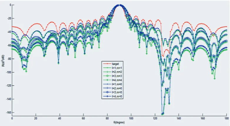
In Figure 6, comparisons between the formed patterns ofl= 1,m= 1;l= 2,m= 2; l= 3,m= 3;

l = 4,m = 4 and l= 1, m = 0; l= 2, m = 0; l = 3, m= 0; l = 4, m= 0 are conducted to show the strength of parameterm. It can be learned from Figure 6 that parametermcan lower the levels of side lobes and null beam to a small extent compared with the counterpart cases of m = 0. For example, whilel= 1m= 1,l= 2 m= 2,l= 3 m= 3,l= 4 m= 4, the null beam minimum levels are−61.5 dB,

−95 dB, −120 dB, −165 dB in turn. However, while l = 1 m = 0, l = 2 m = 0, l = 3 m = 0, l = 4

m= 0, the null beam minimum levels are −59 dB, −89 dB, −118 dB,−161 dB in sequence. From these data, it can be concluded that parameter lhas more effects on outcomes than m.

5. DISCUSSION

Figure 6. The outcomes of non-uniform array simulation; In the column of legend, target denotes the expected beam pattern, LS refers to the pattern formed by the traditional least square solution of Equation (9), l= 1, m = 1; l= 2, m= 2; l= 3, m= 3; l= 4, m= 4 and l= 1, m= 0; l = 2, m= 0;

l= 3,m= 0; l= 4, m= 0 mark the patterns created by the element excitation of Equation (22).

be well used for linear array. However, for other geometry arrays, matrix A may be a two-dimension function of the azimuth angle variable φ, and elevation angle variableϕ and P may be a matrix. The solution cannot be obtained from matrixAandP as mentioned before. In the two-dimension case, how to apply Equation (22) is still a subject of study needed to further investigate.

It is well known that in practice the mutual couplings between the array elements have effects on the real pattern. Mutual coupling of array elements depends on many factors of the array, such as the element shape, element distribution, and element spacing, which are all not considered in the derivation of the new approach. Hence, in practice, the solution of the new method must be modified to adapt the need of the real specific use according to real used array features.

We have simulated arrays with 33, 19, 15, 11, 21, 37, 41 elements. The outcomes show the same conclusion as that of this paper, i.e., in Equation (22), parameter l has more effects on outcomes than

m. We think that this may be caused by the projection space’s characteristic. The mathematical reason forl and m’s effects on outcomes still needs to be studied further in future.

In order to estimate the computational complexity, we consider Equation (15) which is the simplest solution of the new method and Equation (11) which is the solution of the traditional least square method. because P in Equation (11) and D in Equation (15) cause proportional computing volume, it can be concluded that compared with the traditional least square method, the new approach does not increase computational complexity when Pand D are with the same power. We simulate the new approach on a HP notebook PC with core i5-5200U CPU, 4G memory and MATLAB software platform. All simulations in this paper take about one second to get the final outcomes.

In addition, when the array manifold matrix and target pattern are determined in advance, the solution of the new approach can be obtained directly from Equation (22). This merit may make it convenient for the real time processing application.

6. CONCLUSION

and local peak distribution, and is better in the key performance indicators of peak level of side-lobe and null beam level than the targeted pattern. In Equation (22), the integer variable l can affect the synthesized results better thanm.

ACKNOWLEDGMENT

This work has been supported in part by the National Natural Science Foundation of China with No. 61501340 and Department of Education of Shaanxi Province under the Natural Science Fund No. 2017JK1681.

REFERENCES

1. Ohira, T., “Adaptive array antenna beamforming architectures as viewed by a microwave circuit designer,”Proc. Asia-Pacific Microw. Conf., 828–833, Sydney, Australia, Dec. 2000.

2. Denno, S. and T. Ohiro, “Modified constant modulus algorithm for digital signal processing adaptive antennas with microwave analog beam-forming,”IEEE Trans. Antennas Propag., Vol. 50, No. 6, 850–857, Jun. 2002.

3. Sarkar, T. K., J. Koh, R. Adve, et al., “A pragmatic approach to adaptive antennas,”IEEE Acoust., Speech, and Signal Processing Mag., Vol. 42, No. 2, 39–55, Feb. 2000.

4. Chen, Y., S. Yang, and Z. Nie, “The application of a modified differential evolution strategy to some array pattern synthesis problems,”IEEE Trans. Antennas Propag., Vol. 56, No. 7, 1919–1927, Jul. 2008.

5. Manica, L., P. Rocca, M. Benedetti, and A. Massa, “A fast graph-searching algorithm enabling the efficient synthesis of sub-arrayed planar monopulse antennas,”IEEE Trans. Antennas Propag., Vol. 57, No. 3, 652–663, Mar. 2009.

6. He, H., P. Stoica, and J. Li, “Wideband MIMO systems: Signal design for transmit beampattern synthesis,”IEEE Transactions on Signal Processing, Vol. 59, No. 2, 618–628, 211.

7. Oliveri, G., M. Carlin, and A. Massa, “Complex-weight sparse linear array synthesis by Bayesian compressive sampling,”IEEE Trans. Antennas Propag., Vol. 60, No. 5, 2039–2326, May 2012. 8. Chen, H., Q. Wang, and R. Fan, “Beampattern synthesis using reweighted l1-norm minimization

and array orientation diversity,” Radioengineering, Vol. 22, No. 2, 602–609, Jun. 2013.

9. Choi, W., T. K. Sarkar, H. Wang, and E. L. Mokole, “Adaptive processing using real weights based on a direct data domain least squares approach,” IEEE Trans. Antennas Propag., Vol. 54, No. 1, 182–191, Jan. 2006.

10. Zhang, X.,Modern Signal Processing, Tsinghua University Press, Beijing, 2012.

11. Caorsi, S., F. De Natale, M. Donelli, D. Franceschini, and A. Massa, “A versatile enhanced genetic algorithm for planar array design,” Journal of Electromagnetic Waves and Applications, Vol. 18, No. 11, 1533–1548, 2004.

12. Massa, A., M. Donelli, F. De Natale, S. Caorsi, and A. Lommi, “Planar antenna array control with genetic algorithms and adaptive array theory,” IEEE Trans. Antennas Propag., Vol. 52, No. 11, 2919–2924, 2004.

13. Donelli, M. and P. Febvre, “An inexpensive reconfigurable planar array for Wi-Fi applications,”

Progress In Electromagnetics Research C, Vol. 28, 71–81, 2012.

14. Wang, B.-H. and Y. Guo, “Frequency-invariant and low cross-polarization pattern synthesis for conformal array antenna,” IEEE Radar Conf., 1–6, May 26–30, 2008.

15. Comisso, M. and R. Vescovo, “Fast co-polar and cross-polar 3D pattern synthesis with dynamic range ratio reduction for conformal antenna arrays,”IEEE Trans. Antennas Propag., Vol. 61, No. 2, 614–626, Feb. 2013.

17. Khzmalyan, A. D. and A. S. Kondrat Yev, “Phase-only synthesis of antenna array amplitude pattern,” Int. J. Electron., Vol. 81, No. 5, 585–589, 1996.

18. Vaskelainen, L. I., “Constrained least-square optimization in conformal array antenna synthesis,”

IEEE Trans. Antennas Propag., Vol. 55, 859–867, Mar. 2007.