Characterization of Linear Electromagnetic Observables in Stochastic
Field-to-Wire Couplings
Ousmane O. Sy1, 3, *, Martijn C. van Beurden1, and Bastiaan L. Michielsen2
Abstract—This article presents a method to characterize stochastic observables defined by induced surface currents and fields in electromagnetic interactions with uncertain configurations. As the covariance operators of the stochastic distributions and fields are not compact, a strict Karhunen-Lo`eve (KL) approach is not possible. Instead, we apply a point-spectrum regularization by expanding the stochastic quantities on a finite-element-like basis. The coefficients of the KL expansion are approximated analytically in a polynomial-chaos (PC) expansion. The novelty of our approach resides in its ability to handle multiple PC expansions simultaneously and determine the orders of the KL and PC expansionsadaptively. This method is illustrated through the example of the voltage induced at the port of a random thin-wire frame illuminated by random plane waves. The results show the accuracy and computational efficiency of the proposed method, which provides a complete characterization of the randomness of the observable.
1. INTRODUCTION
Electronic systems have to properly function in a vast range of operational scenarios. For example, electronic systems have different compositions due to customer wishes and upgrades over time. This generates many uncertainties in the operational conditions of the system. Other types of uncertainties that occur are ageing and drift, production tolerances, and locations of cable trees due to individual decisions taken by an installer of a system. Under all such conditions, which are partly outside the control of the manufacturer, the manufacturer has to guarantee safe and proper functioning, as well as EMC compliance of the system. Since the number of potential scenarios and deviations from the ideal system is vast, it is rapidly becoming unpractical or impossible to guarantee the proper functioning of a system based on a limited set of deterministic simulations and well-controlled experiments that are induced by practical time and budget constraints.
Research in stochastic electromagnetic fields approaches this dilemma from a different perspective. By introducing uncertainties in a setup from the start, one aims at generating a sufficiently rich stochastic ensemble that will properly represent the entire range of device variations and operational conditions [1, 2]. This rationale has been adopted in reverberation-chamber measurements, where a rich set of electromagnetic fields impinges upon a device under test [3, 4]. A similar train of thoughts can be observed in the construction of numerical methods for CAD tools [5].
Popular methods to analyze stochastic systems are the Monte-Carlo method and Stochastic Collocation, both of which use an underlying parameterized deterministic model and a sampling scheme guided by the assumptions on the probability density functions of the parameters [6–9]. The advantage is that the deterministic model is tackled with well-established numerical methods and that this model
Received 30 June 2016, Accepted 2 October 2016, Scheduled 14 October 2016 * Corresponding author: Ousmane Oumar Sy ([email protected]).
1 Department of Electrical Engineering, Eindhoven University of Technology, Den Dolech 2, 5600 MB, Eindhoven, The Netherlands. 2 ONERA — DEMR, BP 74025, 2, av. Edouard Belin, 31055 Toulouse Cedex 4, France. 3 Now at Jet Propulsion Laboratory,
can be treated as a black box that produces responses for the sampled parameters. Nevertheless, a single model evaluation can already be time-consuming and a sampling approach readily requires several hundreds or thousands of evaluations. Therefore, economizing on the number of model evaluations is an important aspect in constructing numerical tools for stochastic problems.
In the present paper, we address electromagnetic-scattering problems with stochastic parameters in both configuration and excitation field. As in previous papers, the Lorentz reciprocity theorem allows us to compute an observable, e.g., an induced voltage, for multiple excitation fields by solving a linear system for a single right-hand side per variation in the configuration [10, 11]. To allow for the computation of an observable for stochastic excitations and simultaneously avoid the construction of extensive libraries of numerical solutions, we exploit a Karhunen-Lo`eve (KL) decomposition of the essential stochastic distributions and fields [12, 13]. To ensure that the KL expansion can be derived, i.e., that the covariance operators of the fields and currents are compact, the stochastic processes are expanded on finite-element basis functions. The KL decomposition provides a method for determining the degrees of freedom in the problem while a polynomial-chaos (PC) expansion leads to a rapidly converging approximation of the observables as functions on the probability space [14, 15]. We apply the PC expansion semi-intrusively, i.e., instead of applying the PC expansion directly to the induced voltage, we expand the fields and currents that define the voltage, thereby achieving computational gains. By aiming to fully characterize the randomness of the observable, this article extends previous efforts where the semi-intrusive approach was used to determine only the mean and variance of the observable [3, 16].
The general practice is to truncate the KL expansion based on the decay of the eigenvalues of the covariance and use a fixed order for the PC expansion based on its variance. Both choices guarantee the root-mean-square accuracy but not the accuracy of the full distribution. We address these issues by using a higher-order statistic, viz. the Kolmogorov-Smirnov statistic of a canonical voltage, to jointly and adaptively determine theorders of the KL and PC expansions. The required steps in the recipe are made explicit and we demonstrate that the combination of the techniques results in a versatile and powerful scheme. As such, our algorithm focuses on an adaptivep-refinement of the PC expansion, rather than adaptive h-refinement methods proposed in the multi-element probabilistic collocation method [8], or the hierarchical sparse-grid collocation method [9].
The outline of this article is as follows. Section 2 describes the test case used as a prototype to study linear electromagnetic interactions, i.e., a randomly shaped thin-wire frame connected to a random impedance and illuminated by plane waves. Section 3 presents the stochastic model that is sought and built using Karhunen-Lo`eve and polynomial-chaos spectral expansions. The adaptive scheme devised to ensure the joint convergence of the KL and PC expansions is described in Section 4 and illustrated in Section 5 through the KLPC expansion of the current flowing on the random thin-wire frame. The KLPC model is then used in Section 6 to accurately approximate the probability distribution of the voltage induced at the port of the setup by deterministic or random incident fields. The computational cost of the KLPC approach is discussed in Section 7.
2. STOCHASTIC LINEAR-INTERACTION PROBLEM
This section describes a stochastic linear electromagnetic interaction problem involving a thin-wire setup. Thin-wire structures play an important role in antenna theory and in electromagnetic compatibility (EMC) due to their presence in harnesses and cables that interconnect electronic devices. At high frequencies, these wires even behave as radiating elements that must be accounted for to properly describe the total electromagnetic field.
2.1. Definition of the Interaction Geometry
z
x
1 cm
y
1 m
5 cm
β
θ
η E
φ 1 cm
V Z
Wα
y ym
yM
x (y)
z (y)α
α
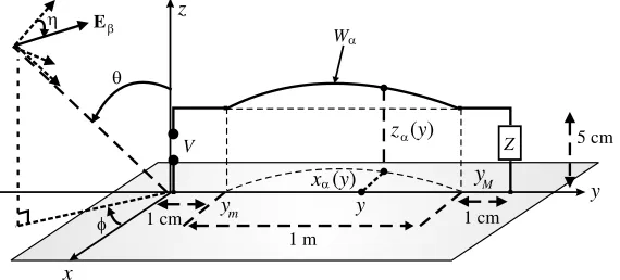
Figure 1. Interaction configuration: perfectly conducting thin-wire frame Wα connected to a load Z
and located above a ground plane, incident fieldEβ and observable V induced at the port ofWα.
The shape of W results from the geometrical deformation of a reference transmission line W0 located 5 cm above a PEC ground plane. The axis of W is defined with respect to W0 through the smooth mapping
τα(r0) =r0+ ⎧ ⎪ ⎨ ⎪ ⎩
(αxux+αzuz) sin
πy0−ym yM −ym
, ify0∈[ym, yM],
0, otherwise,
(1)
for anyr0 = (x0, y0, z0)∈W0, with (ux,uy,uz) the Cartesian basis. The geometrical deformations are
controlled by the vector α= (αx, αz), which belongs toA=Ax× Az, withAx=Az= [−0.03; 0.03] m. To mark the dependence ofW onα, the deformed wire is written asWα. The impedance of the wire is
Z =R+jξ with a deterministic resistance R = 50 Ω and a reactance ξ ∈ X = [−5,5] Ω. Geometrical uncertainties of the setup correspond to an indetermination of α in A, while material uncertainties translate in an indetermination of ξ inX. The consequences of these uncertainties can be severe when dealing with a resonant structure such asWα, as will be shown in Section 2.3.1.
To quantify these uncertainties, a stochastic framework is adopted by gathering the uncertain parameters of the configuration in the vector γ = (α, ξ) ∈ G =A × X and by regarding the variations of γ inG as random. Specifically, γ is a random vector, which has mutually statistically independent components and follows the probability distribution PG that is known a priori or derived from the observations of realizations of the system.
2.2. Definition of the Incident Field
The externally generated incident field is denoted Eβ where β ∈ B ⊂ Rm gathers parameters such as the amplitude, polarization and direction of propagation of the field. This field is assumed to have a plane-wave spectrum, denotedEβ, with
Eβ :R3 r−→
S
Eβ(ki)e−jki·rd3k
i ∈C3, (2)
whereS = 2λπui, with ui ∈R3, ui= 1is the set of wavevectors andEβ(ki)∈C3is the polarization vector, with Eβ(ki)·ki= 0, for any ki∈ S. The support ofEβ in S defines the directions of incidence
(θi, φi) in polar coordinates. For our purposes, the incident fields are assumed to impinge from the
directions (θ, φ) ∈ [0, π/2] ×[−π/2, π/2], i.e., S = {(2π/λ)ur(θ, φ), θ∈[0, π/2], φ∈[−π/2, π/2]},
with
ur(θ, φ) = −(sinθcosφux+ sinθsinφuy+ cosθuz). (3)
2.3. Induced Voltage as Observable
The voltage V induced at the port of the system byEβ is defined as
V(γ, β) =−
∂Wα
Jγ(r)· Eβ(r)dS(r) ∈C, (4)
where the distributionJγ(r) depends solely onγ as it is induced on the mantle ofWαin a transmitting
state, i.e., by a unit current source applied to the port in the absence of Eβ [11]. To accurately account for the deformation of Wα and the boundary conditions at the load Z, Jγ is computed by solving
the electric-field integral equation (EFIE) associated with the transmitting state. The computation and solution of the EFIE impedance matrix are carried out efficiently using an approximate-kernel Pocklington equation [18] and quadratic-segment basis functions [19]. Hence,Jγ is a nonlinear function of γ, each evaluation of which incurs a given numerical cost. Alternative electromagnetic models could have been considered, e.g., based on transmission-line theory [20, 21]. However, one must make sure that these models can properly handle the varying height-above-ground of the thin wire.
2.3.1. Motivation of the Uncertainty Quantification
The electromagnetic behavior of the setup is illustrated in Fig. 2 as a function of frequency for a wire connected to a resistance Z = 50 Ω. The incident field is a parallelly polarized plane wave with an electric field of amplitude 1 V·m−1, propagating along the direction (θ= 45◦, φ=−45◦). This graph shows the amplitude |V| of the induced voltage for the mean configuration αAVG = (0,0) and the
“extreme” deformations obtained with αMAX = [0.03,0.03] m and αMIN= −αMAX. The current Jγ is
computed via a method of moments (MoM) by discretizing the axis of the wire into 224 segments. This produces a uniform mesh with 5 mm long segments.
These plots show resonance peaks in the spectrum of |V|. The effects of the deformations are noticeable through the shift between the resonance frequencies of αAVG compared to those ofαMIN and αMAX. For instance, at f1 = 1997 MHz, if the deformations are ignored, using the response of αAVG
for all configurations can lead to an over-estimation of the voltage by up to 4 dB. Hence, the need for
1900 1950 2000 2050 2100 2150 2200
-14 -13 -12 -11 -10 -9 -8 -7
frequency f [MHz]
voltage |V| [dBV]
f
1= 1997 MHz
αMIN αAVG αMAX
an uncertainty quantification at such a frequency, which is the frequency considered in the remainder of the article.
2.3.2. Stochastic Parametrization of the Voltage
Through Eq. (4), the randomness ofγ orβ induces the randomness ofV. However, unlikeγ orβ, the probability distribution PV of V is unknown. The aim of the stochastic approach is to characterize or approximate PV given PG, PB and the dependence ofV on (γ, β). Due to the numerical and nonlinear dependence ofV on (γ, β),PV cannot be determined analytically.
The distributionPV can be characterized by a Monte-Carlo (MC) approach, viz. by generating a large set of samples of V using values of (γ, β) drawn randomly according to PG and PB. Then, this large dataset can be used to compute statistical moments or approximate the cumulative distribution function (CDF) ofV. However, a drawback of this approach is that whenever eitherPG orPB changes, a new MC analysis is required. Second, the generation of a large MC dataset implies the solution of as many boundary-value problems, which rapidly becomes cumbersome numerically.
To circumvent the first limitation, we reformulate the observable to separate the effects of the geometrical uncertainties from the uncertainties due to Eβ. Next, we apply a spectral expansion to express the dependency of V on γ and β explicitly in terms of polynomials, which in turn eases the statistical processing ofV significantly.
2.3.3. Spectral Reformulation of the Observable
Although Eβ is independent of the scattering device, it must still be evaluated over the support of
Jγ, viz. at a point on the mantle of the wire r ∈ ∂Wα, to compute V. Therefore, the geometrical
modifications of the setup also affect Eβ, thereby complicating the characterization of the variations of Jγ independently from Eβ. This difficulty is avoided by using a spectral definition of V through
Plancherel’s theorem [22, p. 188], i.e.,
V(γ, β) =−
S
Jγ(k)·E∗β(k)d3kdef= − Jγ;EβS, (5)
where (∗) is the complex conjugation andJγ the Fourier transform of Jγ
Jγ:S k−→
∂Wα
Jγ(r)e−jk·rdS(r)∈C3. (6)
The advantage of Eq. (5) over Eq. (4) is that the randomness of the system is now entirely contained in
Jγ and can be quantified by characterizing the randomness of Jγ only. The resulting information can
be re-used to obtain statistics of V, regardless of the type of incident field.
3. STOCHASTIC SEMI-INTRUSIVE KLPC MODEL
3.1. Outline of the Method
In this section, we propose a representation of the stochastic observable to highlight the most efficient way of doing the numerical computations. In the integral representation of Eq. (5), Jγ is a stochastic field defined by the probability spaceG and mapping eachγ ∈ G to the space of infinitely smooth fields with their support inS, which is denoted E(S,C3) [22, p.92]. As forEβ, it is a stochastic generalized function defined by the probability spaceBand valued inE(S,C3), i.e., the dual space ofE(S,C3). The objective is to have a convenient representation of the objects in the definition of the observable to access the dependency of the observable on the stochastic parameters (γ, β). This in turn will significantly ease the evaluation of the statistical properties of V.
We suppose thatJγ has the following approximation
Jγ(k) ≈ N
n=0
where {Jn}n=0,...,N is a set of deterministic vector fields regular in S and {ρn}n=0,...,N is a set of
orthogonal functions defined onGand which will be approximated via polynomials. This approximation, which will be obtained by applying Karhunen-Lo`eve (KL) and polynomial-chaos (PC) expansions described in the next section, yields a model that is henceforth denoted KLPC. Inserting Eq. (7) in (5) leads to
V(γ, β) ≈
N
n=0
ρn(γ)νn(β), with νn(β) =− Jn;EβS. (8)
Equation (8) is already an advantageous representation of the observable whenEβ is cheap to compute, e.g., when it consists of the sum of a small number of plane waves. Indeed, since {Jn}n=0,...,N
are deterministic, they need to be computed only once and statistical operations only involve the polynomials that approximate {ρn(γ)}n=0,...,N, which are easy to evaluate. This way of applying the
PC expansion is semi-intrusive, i.e., intrusive with respect to the final observable that is V, and non-intrusive for Jγ and Eβ as the PC expansion is not applied to the operators that define these two
quantities.
3.2. Stochastic Spectral Model: KLPC Expansion
Without loss of generality, the KLPC expansion is described for Jγ. Since the covariance of Jγ is not necessarily compact, a Karhunen-Lo`eve decomposition cannot be applied stricto sensu. To sidestep this issue, a weak formulation is used by expanding the stochastic processes on a set of deterministic finite-element basis functions, which is denoted H = {h : S −→ R}=1,...,NS and may consist, e.g., of pulses or triangular functions. Expanding all the components ofJγ in terms of these functions leads to
Jγ(k) ≈
NS
=1
Iγ()h(k), (9)
where Iγ() = h;Jγ
S ∈C3, ∀= 1, . . . , NS, (10)
with {h} functions from the bi-orthogonal set of H, i.e., hk;h
S = δk, for any k, , with δk, the
Kronecker symbol. The meanμI and the covariance CI ofIγ ∈C3NS are defined then as
μI() = E[Iγ()] =
G
Iγ()fG(γ)dγ, (11)
CI(, ) = EIγ()I∗γ()
−μI()μI∗(), (12) where E[·] is the expectation operator with respect to γ, and fG is the probability density function (PDF) ofγ. In practice, the right-hand sides (rhs) of Eqs. (11)–(12) are computable by quadrature, as discussed in Section 5.1.
Then, using the eigenvalues λ1 ≥ . . . ≥ λ3NS ≥ 0 and the eigenvectors {ϕn}n=1,...,3NS of CI, a
Karhunen-Lo`eve (KL) expansion is applied toIγ, which leads to [6, p. 17]
Iγ() = μI() +
3NS
n=1
λnρn(γ)ϕn(), ∀γ ∈ G, (13)
where, for any n≥1, the normalized KL variables
ρn(γ) =
1
√ λn
Iγ−μI;ϕnS (14)
are centered, with unit variances and mutually uncorrelated. Owing to the generally rapid decay of the eigenvalues λn, the sum in Eq. (13) can be truncated to a low orderNKL 3NS and still yield a very
accurate approximation ofIγ in theL2 sense,
Iγ() ≈ μI() + NKL
n=1
ρn(γ)
By introducingρ0 = 1, λ0 = 1, ϕ0 =μI and Jn(k) =
√ λn
3NS
=1
ϕn()h(k), one obtains a representation
of the form (7), i.e.,
Jγ(k) ≈ JNKL
γ (k) =
NKL
n=0
ρn(γ)Jn(k). (16)
To completely characterize the randomness of JNKL
γ , one needs to determine the joint probability
distribution Pρ of ρ= (ρ1, . . . , ρNKL), which are mutually uncorrelated but not necessarily statistically independent. Once Pρ is known, the statistical post-processing of Iγ becomes seamless. If Iγ depends
analytically on γ, Pρ can be determined either analytically or by computing an empirical distribution
at little numerical cost. In our case, whereIγ depends numerically on γ, we apply a polynomial-chaos expansion to expressρ analytically in terms ofγ and thereby ease the estimation of Pρ.
3.2.1. Polynomial-chaos Expansion
Since all the components of ρ have finite variances, they can be expanded on a basis of orthogonal polynomials [6]. In addition to offering explicit analytical expressions of the random processes in terms of γ, polynomials have the advantage of an exponential convergence for functions that are infinitely differentiable. Hence,
ρ(γ) =
m∈Nd
c(m)ψdm(γ), ∀= 1, . . . , NKL, (17)
with c(m) = E
ρ(γ) ψmd(γ)
. (18)
The polynomials {ψmd(γ)}m are d-variate, with d the dimension of G, and mutually orthogonal with respect to the inner product defined by fG, i.e., Eψdm(γ)ψmd(γ)
= δmm, for any m,m ∈ Nd [23]. Eq. (18) shows that the computation of every c(m) requires the availability of ρ(γ) and a sampling
strategy in G. Trying to compute the PC coefficients c(m) by quadrature breaks down rapidly as
the order of the polynomials ψdm(γ) or the dimension of G increase. Higher PC orders are difficult to compute due to the finite degree of polynomial exactness of the integration rules, while increasing the dimension G leads to a curse of dimensionality. Instead, since Eq. (17) is a linear equation in c(m),
it is solved for the PC coefficients using least-squares linear regression [24], as detailed in Section 4.1. Moreover, since the coefficients {c(m)},m are deterministic, they can be pre-computed, stored and re-used for other incident fields.
For practical-implementation purposes, Eq. (17) is truncated to a finite order. We choose to apply an isotropic truncation by using the same order NPC for all univariate polynomials and for all the KL
variables, i.e.,
ρ(γ)≈ NPC
m=0
c(m)ψmd (γ) =
Ncoeff
j=1
c[m(j)]ψmd(j)(γ), (19)
where c(m) = [c1(m), . . . , cNKL(m)], Ncoeff = (NPC+ 1)d is the number of PC coefficients, and the
multi-indices are numbered through the bijection
{1, . . . , Ncoeff} j−→m(j)∈ {0, . . . , NPC}d.
3.2.2. KLPC Expansion of the Current Jγ
The KLPC approximation of Jγ, derived from Eqs. (19) and (16), reads
Jγ ≈
NKL
n=0
NPC
m=0
This approximation captures the spatial dependency of Jγ deterministically via the eigenfunctions of
the covariance, and the randomness of Jγ analytically through the PC approximation of ρ. Since the KLPC model is analytical, Pρ can be estimated by generating a large ensemble of samples of ρ at a
negligible numerical cost.
4. ADAPTIVE IMPLEMENTATION OF THE KLPC MODEL
With the stochastic model now established, two major aspects need to be considered, viz. 1) the method for computing the PC expansion, and 2) the method for determining the orders of the KL and PC expansions to ensure the accuracy of the resulting KLPC probability distribution.
4.1. Estimated Accuracy of the PC Expansion for a Fixed KL Order
Since Eq. (19) is linear inc(m), the PC coefficients are computed by least-squares (LS) linear regression. For a given KL expansion of order NKL, the LS problem is formulated as
ΨPC(GReg) CKP = P(GReg), (21)
with GReg = {γk}k=1,...,NReg ⊂ G the regression set, ΨPC(GReg) =
ψdm(j)(γi)
1≤i≤NReg,1≤j≤Ncoeff and CKP = (c[m(j)])1≤≤NKL;1≤j≤Ncoeff the KL coefficients to be determined. The rhs P(GReg) = [ρj(γi)]1≤i≤NReg,1≤j≤NKL is evaluated using Eq. (14). Solving Eq. (21) forCKP yields the estimate
CKP≈
ΨtPCΨPC
†
ΨtPCP, (22)
with (†) the pseudo-inverse operator. Only one inversion of ΨPCis required for every setGReg. Increasing NKL only increases the dimension of P(GReg) while leaving ΨPC(GReg) (to be inverted) unchanged.
Thus, our algorithm is rather insensitive to the number of KL variables, which is advantageous for the parallelized computation of multiple PC spectra. To ensure the accuracy of the estimate, and given our limit to the number of function evaluations (NMAX), we conservatively use 3Ncoeff samples in the
LS algorithm as long as 3Ncoeff ≤NMAX, otherwise we use 2Ncoeff samples as long as 2Ncoeff ≤NMAX.
Hence, the highest PC order that can be considered is
NPC,max=
NMAX
2
1/dim(G)
−1
. (23)
The power of a PC approximation of order NPC, viz.
N3(c) =
Ncoeff
j=1
|c[m(j)]|2 (24)
is compared to 1, i.e., the theoretical variance ofρ. Thus, given a toleranceεPC,max, the KL coefficients
that verify |N3(c)−1| ≤ εPC,max are assumed to be sufficiently accurately approximated by the PC
expansion.
4.2. Adaptive KLPC Decomposition
It is common practice to truncate the KL approximation based on the decay of the eigenvalues of CI. For instance, given a threshold τKL > 0, one finds the order NL2 as the smallest integer such that
k>NL2
λk
k≥1
λk < τKL. While such an approach ensures the accurate restitution of the variance of
the observable to within τKL, it does not guarantee the accuracy of higher-order moments. To tackle
MKL →
MKL+1
If MKL> NL2
where for every PC order MPC, the PC
coeffs {cl} are computed by r egression
Build the canonical voltage Vtst(MKL)
Compute the CDFFtst(MKL) of Vtst(MKL)
MKL= NL2-1 Initialization
Compute the Kolmogorov-Smirnov statistic
If MKL=NL2
If k(MKL) >εmax2
If k(MKL) <=εmax2
Optimal KL order: NKS= MKL
Optimal PCorder: NPC=
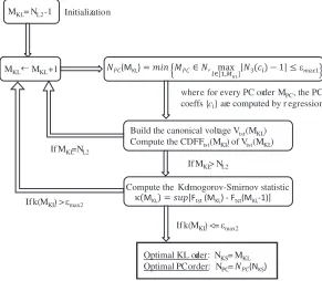
Figure 3. Flow-chart showing the adaptive determination of the orders of the KL and PC expansions.
First, the PC expansion is computed for MKL = NL2 KL variables. The accuracy of the PC
approximation of the coefficients c is assessed by verifying that|N3(c)−1| ≤εPC,max (see Eq. (24)),
for a given toleranceεPC,max. Next, the canonical variable
Vtst(MKL) =
MKL
n=1
λn|ρn(α)|2 ≥0 (25)
is considered. This variable can be regarded as the voltage induced on a wire on which flows the current
Jα−μJ by an incident field Etst =
MKL
n=1
ρ∗n(α)ϕ∗n. The CDF of Vtst(MKL), denoted FMKL, is readily available via sampling the PC expansion. This procedure is then repeated forMKL←MKL+ 1 and the
CDFs FMKL and FMKL−1 are compared using the Kolmogorov-Smirnov (KS) statistic [25, p. 316] κ(MKL) = sup
v≥0|FMKL
(v)−FMKL−1(v)|. (26)
This quantifies the difference in higher-order statistics due to the increasing order of the KL expansion. The value of MKL is incremented until κ(MKL) drops below a threshold εKS chosen by the modeler.
The resulting optimal KL order is denoted NKS. It is worth noting that, whenever MKL is increased,
the order of the PC expansion is increased until allMKLKL variables are accurately expanded following
the rationale of Section 4.1.
The numerical efficiency of this approach hinges on two choices that we make. First, since our implementation of the PC-projection algorithm is insensitive to the number of KL variables being computed (see Section 4.1), we simultaneously compute the PC projections of multiple KL variables with the same regression setGReg. Our second choice is motivated by the fact that solving Eq. (21) every
time the KL or PC orders are increased can become numerically cumbersome. Instead, we compute the PC spectra of a super-set of MKL,max KL variables simultaneously and verify the accuracy of the
subset of MKL variables of interest. Only when the MKL variables are not accurate in RMS sense (i.e.,
there is at least one ∈ {1, . . . , MKL} such that |N3(c)−1| > εPC,max) is the order NPC increased
and the PC projection recomputed, by LS regression, for the super-set ofMKL,max KL variables. Both
the best of the authors’ knowledge, this is a novel approach to perform KL and PC expansions jointly and adaptively.
5. KLPC EXPANSION OF THE CURRENT DISTRIBUTION
We now apply our KLPC method to the stochastic thin-wire setup described in Section 2.1. We recall that this problem involves three random parameters, viz. γ = (αx1, αz1, ξ), which are assumed
mutually statistically independent with uniform distributions in their ranges. To apply the spectral reformulation at the core of our stochastic method, the domain S is sampled into the wave-vectors
ki,= (2π/λ)ur(θi, φ) (see Eq. (3)), with
θi = arccos
i N1
, φ= π
2
−1
N1 −
1
, (27)
where i = 1, . . . , N1−1 and = 1, . . . ,2N1 + 1 with N1 = 10. This results in a discrete sampling of S into Ndir = (N1 −1)(2N1 + 1) = 189 directions of incidence. The expansion and testing functions
({h} and{h}) overS are chosen as delta functions and the functions defined onS are approximated
by point-matching, i.e., Eβ(ki,) and Jγ(ki,) are represented by (3Ndir)-dimensional vectors. As an
indication, using the deterministic model with the axis ofWα subdivided intoNseg= 224 segments, the
computation of the voltage induced by a single plane wave (the superposition of all Ndir plane waves)
requires ∼ 218 ms (∼340 ms) on a 2.7 GHz computer with an Intel Core i7 processor. Thus, most of the computational effort is devoted to the build-up of the impedance matrix in the MoM and its LU factorization.
5.1. Second-Order Statistical Moments
The meanμI and covarianceCI in Eqs. (11) and (12) are computed using a sparse-grid (SG) quadrature rule, which is well suited to handle integrals over multi-dimensional domains and takes advantage of the smoothness of the integrands [26]. As a reference, a Monte-Carlo (MC) algorithm is also used. Both of these quadrature rules are known to mitigate the effects of the “curse of dimensionality”, i.e., the exponentially-growing complexity as a function of the dimension of the sampling space. More advanced sampling schemes, e.g., with adaptive dimensionality reduction, could also be considered [8, 9].
Since CI is a higher-order moment than μI, its computation is more demanding. Hence, the convergence of the quadrature estimates is monitored through the relative variations of CI in terms of its Fr¨obenius norm [27, p. 55], as the complexity of the quadrature increases. Table 1 shows the relative error ofCI versus the complexityNquadof the quadrature rule. For both algorithms,CIcan be obtained
with a relative accuracy better than 0.1% (even ∼0.01% for the SG rule) with ∼103 samples.
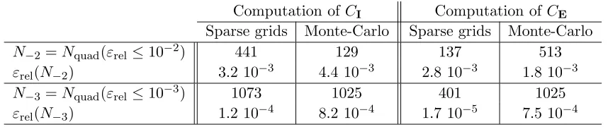
Table 1. Convergence of the Monte-Carlo and sparse-grid estimates of the covariance matrices CI (random geometry) and CE (random incident field studied in Section 6.2). Number N−k of function
evaluations required to reach target accuracy εrel ≤εmax= 10−k, and relative errorεrel(N−k).
Computation ofCI Computation of CE Sparse grids Monte-Carlo Sparse grids Monte-Carlo
N−2 =Nquad(εrel ≤10−2) 441 129 137 513
εrel(N−2) 3.2 10−3 4.4 10−3 2.8 10−3 1.8 10−3
N−3 =Nquad(εrel ≤10−3) 1073 1025 401 1025
εrel(N−3) 1.2 10−4 8.2 10−4 1.7 10−5 7.5 10−4
Next, CI is spectrally decomposed using an eigenvalue solver (e.g., F02GCF of the LAPACK library) [27, p. 393]. The numerical cost of this decomposition scales as∼(3Ndir)3 and requires∼12 s.
5.2. KLPC Decomposition of Jγ
Since all the random input parameters in this article follow a uniform probability distribution, it is natural to consider a Legendre-uniform polynomial chaos [28]. The Legendre polynomials are obtained recursively [23, p.333]. The orders of the KL and PC expansions are determined adaptively according
Table 2. Main eigenvalues of the covarianceCI normalized by Tr(CI) (left two columns), and similarly forCE (right two columns)
Eigenvalues ofCI Eigenvalues ofCE
with Tr(CI) = 1.652 (A·m−1)2 with Tr(CE) = 5.827 10−3(V·m−1)2 k λ2k/Tr(CI) 1−
k
=1
λ2/Tr(CI) λ2k/Tr(CE) 1− k
=1
λ2/Tr(CE) 1 9.810 10−1 1.903 10−2 5.912 10−1 4.088 10−1 2 1.571 10−2 3.324 10−3 4.085 10−1 2.776 10−4 3 2.069 10−3 1.255 10−3 2.142 10−4 6.338 10−5 4 1.236 10−3 1.860 10−5 4.754 10−5 1.585 10−5 5 1.207 10−5 6.523 10−6 1.288 10−5 2.965 10−6 6 4.951 10−6 1.572 10−6 2.863 10−6 1.020 10−7 7 8.582 10−7 7.138 10−7 4.170 10−8 6.031 10−8
1 2 3 4 5 6 7 8 9 10 11 12 13 14 15 0.6
0.7 0.8 0.9 1 1.1 1.2
k: index of the KL variable ρ
k(γ)
std dev. of PC spectrum
N L2 = 4
N
PC = 2: Ncoeff = 8, NReg = 26
N
PC = 3: Ncoeff = 27, NReg = 82
N
PC = 4: Ncoeff = 64, NReg = 194
N
PC = 5: Ncoeff = 125, NReg = 376
N
PC = 6: Ncoeff = 216, NReg = 650
1 2 3 4 5 6 7 8 9 10 11 12 13 14 15 10-3
10-2 10-1
NKL: order of the KL expansion
K.S. statistic of V
tst
(N
KL
)
N L2 = 4
(a)
(b)
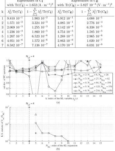
Figure 4. Variance- and KS-based adaptive determination of the KL and PC orders for Jγ: (a) variances of the first 15 KL variables as a function of the order NPC of the PC expansion. (b) Value of
to the scheme described in Section 4.2. Thus, we simultaneously compute the PC spectra of a superset consisting of the firstMKL,max= 15 KL variables, i.e., more than the NL2 = 4 variables prescribed by
the decay of the eigenvalues. Since dim(G) = 3 (i.e., γ = (αx
1, αz1, ξ)) and given our limit to the number
of function evaluations of NMAX= 2000, Eq. (23) indicates that the highest order of PC expansion we
can consider isNPC,max= 9.
The top part of Fig. 4 displays the variances of the KL variables after applying PC expansions of increasing orders. The number Ncoeff of PC coefficients per KL variable is indicated in the legend,
as well as the number NReg of samples used to estimate the PC coefficients by LS regression. After
every PC expansion, the variance of each KL variable is compared to its theoretical value of 1, with a maximum tolerance of εPC,max= 0.1. One could consider a tighter threshold at the expense of a larger
computational burden. With these criteria, according to Fig. 4(a), to estimate the first NL2 = 4 KL
variables accurately, one needs to use NPC = 3, since for NPC = 2 the variance of ρ1 is 1.145 and the
deviation from 1 is larger than εPC,max. Once the NL2 variables are accurately determined, they are
used to build the CDF of the canonical voltage Vtst(NL2), which is stored.
Next, the number of KL variables is increased to MKL = NL2 + 1 = 5. As the variances of {ρ1, . . . , ρ5} are already accurate with NPC = 3, a new PC projection is not required and these PC
coefficients can be used to obtain the CDF of Vtst(MKL) and compute the corresponding KS statistic κ(MKL), which is shown in Fig. 4(b) and equal to 3 10−3. Since this value is larger than the threshold εKS = 10−3, more KL variables must be included in the analysis, and therefore MKL is increased to NL2+ 2 = 6.
The process described in the previous paragraph is iterated and, as shown in Fig. 4, it converges when NKS = 10 KL variables are included in the KL expansion, for which one needs a PC expansion
of order NPC = 6 (mainly due to the slow convergence of the PC expansion of ρ6). This amounts to Ncoeff = 216 PC coefficients per KL variable, for which we use NReg = 650 random samples in the
least-squares estimation process.
With the KLPC expansion at hand, the probability distributionPρ of the vector of dominant KL
variables ρ = (ρ1, . . . , ρNKS) is approximated via Eq. (19) by generating a large set of samples ofρ at minimal cost: for instance, computing 104 samples forρ requires merely ∼2 s.
6. VOLTAGE INDUCED BY ARBITRARY INCIDENT FIELDS
The KLPC model is now used to estimate the PDF of the voltage induced at the port of the wire by arbitrary combinations of plane waves with their supports inS. Using Eq. (2), the polarizations of the incident fields are defined as the following Gaussian beams [29]
Eβ(ki, η) = ωβ(ki)E0[ed(ki, η) +em(ki, η)], ∀ki∈ S, (28)
withE0= 1 V·m−1, andηthe polarization angle of the incident field. The unit vectored(ki, η) indicates
the polarization of the “direct” plane wave, i.e., propagating along the directionki, with a polarization
angleη. Similarly, em(ki, η) is a unit vector directed along the polarization of the mirror-imaged plane wave induced by the presence of the PEC ground plane. The Gaussian weighting function ωβ is given
by
ωβ(ki) = ω0exp
− 1
2σ0
|ki×k0|2 |ki·k0|2
, (29)
withk0 = (2π/λ)ur(θ0, φ0) the mean wave-vector, σ0 the width, and ω0 a normalizing factor such that
the integral ofωβ over S equals 1.
6.1. Deterministic Incident Fields
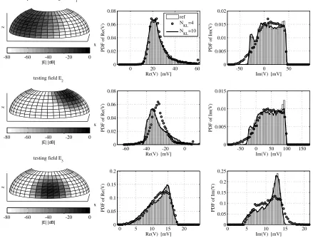
• Field E1: a combination of parallel-polarized (η = 90◦) waves, centered around (θ0 = 60◦, φ0 = −45◦), with a width σ0 = 0.2;
• FieldE2: a combination of parallel-polarized (η= 90◦) waves, centered around (θ0= 45◦, φ0 = 45◦),
with a widthσ0 = 0.1;
• FieldE3: a combination of perpendicular-polarized (η = 0◦) waves, centered around (θ0= 45◦, φ0 =
0◦), with a width σ0 = 0.1.
The amplitudes of these fields are plotted in Fig. 5 (left column). For each of these incident fields, the PDFs of the real and imaginary parts of the induced voltage V are determined using 1) a set of
Nemp = 104 random realizations of the deterministic model (i.e., by evaluating Eq. (4)) and taking
this set as a reference, 2) the L2-based KLPC expansion that uses N
L2 = 4 KL variables, and 3) the
higher-order KL expansion that usesNKS = 10 KL variables. The results, plotted in Fig. 5 (middle and
right columns), show the varying levels of accuracy of the L2-KLPC model depending on the incident field. For instance, with E1 or E3, the L2-KLPC expansion yields an accurate approximation of the
distribution of Re(V). However, differences can be noted in the shapes of the PDF of Re(V) induced by
E2, and the PDFs of Im(V). In contrast, the higher-order KLPC approximation is accurate in terms
of the shape and the support of the PDFs of Re(V) and Im(V).
The KLPC approach is also advantageous for its computation time as shown in Table 3: once the initial effort has been devoted to building the KLPC model (in ∼ 13 mins), subsequent uses of this
x y
Amplitude of testing field E1
z
|E| [dB]
-80 -60 -40 -20 0
0 20 40 60
0 0.02 0.04 0.06 0.08
Re(V) [mV]
PDF of Re(V)
ref NKL=4 NKL=10
-50 0 50
0 0.005 0.01 0.015 0.02
Im(V) [mV]
PDF of Im(V)
x y
testing field E2
z
|E| [dB]
-80 -60 -40 -20 0
-60 -40 -20 0 0
0.02 0.04 0.06 0.08
Re(V) [mV]
PDF of Re(V)
-50 0 50 100 150 0
0.005 0.01 0.015
Im(V) [mV]
PDF of Im(V)
x y
testing field E3
z
|E| [dB]
-80 -60 -40 -20 0
0 5 10 15 20
0 0.05 0.1 0.15 0.2
Re(V) [mV]
PDF of Re(V)
0 5 10 15 20
0 0.05 0.1 0.15 0.2 0.25
Im(V) [mV]
PDF of Im(V)
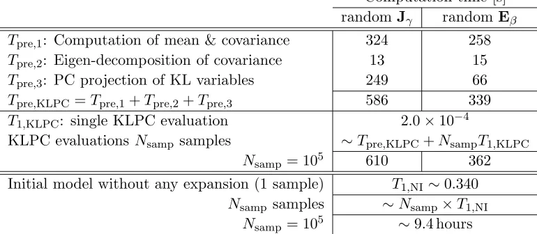
Table 3. Detail of the computation time for the KLPC approach and the systematic use of the initial model (i.e., without the KLPC expansion).
Computation time [s] randomJγ randomEβ
Tpre,1: Computation of mean & covariance 324 258 Tpre,2: Eigen-decomposition of covariance 13 15 Tpre,3: PC projection of KL variables 249 66
Tpre,KLPC=Tpre,1+Tpre,2+Tpre,3 586 339
T1,KLPC: single KLPC evaluation 2.0×10⁻⁴
KLPC evaluationsNsamp samples ∼Tpre,KLPC+NsampT1,KLPC
Nsamp = 105 610 362
Initial model without any expansion (1 sample) T1,NI ∼0.340 Nsamp samples ∼Nsamp×T1,NI
Nsamp = 105 ∼9.4 hours
model come at very little numerical cost (∼2 s to compute the 104 voltage samples per incident field). This is significantly less than the ∼ 30 min required to compute the reference PDF for each incident field via the deterministic model.
6.2. Stochastic Incident Field
The KLPC approach can also be used to characterize a random incident field and determine its interaction with arbitrary receivers. This application is relevant, e.g., for mode-stirred-chamber problems where the field in the test volume is best described as stochastic. Using Eqs. (28) and (29), the stochastic incident fieldEβ considered here has a random amplitudeE0 ∈[0.5,3] V·m−1, a random
polarization defined by the angleη0 ∈[0◦,90◦] and a Gaussian weighting of deterministic widthσ0 = 3
but random mean direction of incidence given by θ0∈[30◦,60◦] and φ0 ∈[−45◦,45◦].
The vector β = (E0, θ0, φ0, η0) of uncertain parameters is assumed random with mutually
independent uniformly distributed components. Although the dimension of β is higher than the dimension of γ = (α, ξ), the dependence of Eβ on β is significantly smoother than the dependence of Jγ on γ at the resonance frequency f1 = 1997 GHz. When computing the meanμE and covariance CE by quadrature, the sparse-grid rule takes advantage of this smoothness, unlike the Monte-Carlo rule, as shown in Table 1 (right two columns containing the results forCE). The smoothness of Eβ in terms of β translates also in a rapid decay of the eigenvalues of CE (see Table 2, right two columns):
NL2 = 2 eigenvalues account for more than 99.9 % of the trace of CE. The KLPC expansion of Eβ is
done adaptively, with a canonical voltage Vtst defined using the eigenvectors and eigenvalues of CE in
Eq. (25). The resulting model comprises NKS = 7 KL variables expressed via a PC expansion of order NPC = 3, i.e., Ncoeff = 81 PC coefficients per KL variable, computed using NLS = 244 samples in the
LS regression.
This KLPC model of the random Eβ is combined with the KLPC model of the random wire of Section 5 to characterize the voltage induced by their mutual interaction. This problem involves seven random parameters, viz. (αx, αz, ξ, E0, θ0, φ0, η0). The KLPC approximations ofJγ and Eβ are
Jγ ≈
NKS,J
n=0
ρJ,n(γ)
λJ,nϕJ,n, Eβ ≈ NKS,E
m=0
ρE,m(β)
λE,mϕE,m, (30)
with ρJ,0 =ρE,0 =λJ,0 =λE,0 = 1, ϕJ,0 =μI, ϕE,0 =μE, and {λJ,n, ϕJ,n}n≥1 and {λE,m, ϕE,m}m≥1
the eigen-systems of CI and CE, respectively. The orders of the KL expansions of Jα and Eβ are
12 14 16 18 20 22 24 26 28 30 0
0.05 0.1 0.15 0.2
|V| [dBmV]
PDF of |V|
24 24.5 25 25.5 26 26.5 27 27.5 28 28.5 29
10-5 10-4 10-3 10-2 10-1
|V| [dBmV]
1
CDF of |V|
ref KL(L2) KL(KS)
(a)
(b)
Figure 6. (a) PDF and (b) complementary CDF of the amplitude of the voltage induced by the random incident field at the port of the random wire, as obtained from 105 samples (ref), the variance based KLPC expansion [KL(L2)] and the adaptive higher-order KLPC expansion [KL(KS)].
inserting Eq. (30) in Eq. (4), i.e.,
V(γ, β)≈ −
NKS,J
n=0
NKS,E
m=0
λJ,nλE,mGJ,E(m, n)ρJ,n(γ)ρE,m(β). (31)
The matrix GJ,E =
ϕJ,n;ϕE,mS
n,m captures the spatial correlation between the two sets of
eigen-functions, while the product λJ,nλE,m acts as a physical weight and the KL variables carry the
randomness.
Another advantage of the Eq. (31) is that with merely NMC random realizations of γ and NMC
random realizations ofβ, one getsNMC2 random realizations ofV, for the computation time required to
run the KLPC models 2NMC times. To keep the problem manageable, we only use 105 samples of the
deterministic model (computed in ∼8.5 hours) as a reference for comparisons against the distributions of VL2 = VNL2,J,NL2,E and VKS = VNKS,J,NKS,E. Fig. 6(a) shows that VL2 already produces an accurate
approximation of the PDF of|V|despite an overshoot at the mode of the distribution, around 23 dBmV. Since the distribution is plotted for|V|on a logarithmic scale, the shape of the distribution is the same for the received power P = |V|2/2 induced at the port of the wire, albeit with a shifted support. As a practical application of the statistics at hand, we determined the probability of exceedance of|V|by analyzing the complementary CDF, i.e., 1−F|V|. Fig. 6(b) illustrates the limited error that is made to
estimate these probabilities of exceedance when using VKS rather than VL2.
7. COMPUTATION TIME
that needs to be invested in only once, followed by evaluations of the thus obtained KLPC model. The pre-computations start with the determination of the mean and covariance operators by quadrature, the efficiency of which depends on the smoothness of the dependence of the integrand with respect to the stochastic parameters. This is well illustrated in Tables 1 and 3, where the slower convergence of the computation of CI compared to CE is due to the rougher behavior of Iγ versus γ caused by the
resonances.
The spectral decomposition of the covariance matrix requires ∼ 14 s for this problem and this cost evolves with the cube of the dimension of the stochastic tensor, i.e., (3Ndir)3. Since the PC
decomposition of the dominant KL variables by linear regression involves a singular-value decomposition, the complexity of this task evolves as ∼ Ncoeff3 = (NPC,1)3dim(G), where NPC,1 is the order of the
univariate PC expansions. All these factors contribute to a total pre-computation time Tpre,KLPC that
ranges from 339 s (∼5.6 min) to 586 s (∼10 min), as reported in Table 3.
After this numerical investment, the evaluations of the KLPC model of the observable merely requireT1,KLPC∼0.2 ms, which is three orders of magnitude smaller than theT1,NI∼345 ms required to
evaluate the observable via the initial model. For instance, generating an ensemble ofNsamprealizations
of the observable will requireNsampT1,NIseconds with the initial model, versusTpre,KLPC+NsampT1,KLPC
seconds in the KLPC approach. Table 3 shows that, already with a single incident field, the KLPC approach outperforms the brute-force approach when it comes to computing the distribution of the induced voltage usingNsamp = 105 samples.
8. CONCLUSION
We have presented a method for characterizing stochastic linear observables that describe electromagnetic interactions between a randomly shaped material object and arbitrary incident fields. The stochastic approach hinges on the accurate computation of the mean and covariance of the stochastic tensors by quadrature, the spectral decomposition of the covariance and the projection on a set of orthogonal polynomials by linear regression. Even though the covariance operators of the electromagnetic fields and current distributions are not compact in general, which is a prerequisite for the spectral decomposition, our method uses a point-spectrum regularization to cast the problem in terms of compact operators. A spectral reformulation of the observable allowed us to separate the effects of the randomness of the scatterer from the randomness of the incident field.
Our implementation of the polynomial-chaos projection is optimized to compute multiple PC projections simultaneously, which makes it a good candidate for parallelization. We have presented an adaptive algorithm to determine the orders of the KL and PC expansions jointly and adaptively using higher-order statistics. Such a rationale refines the common approach that truncates the KL expansion using only the decay of the eigenvalues of the covariance. Our KLPC model provides a complete statistical toolbox to approximate the probability distribution of the observable accurately.
The results obtained for the example of the voltage induced at the port of a stochastic thin-wire frame by arbitrary combinations of plane waves show the high accuracy and numerical efficiency of the proposed method, thereby justifying the numerical investment in the construction of the KLPC model. While this article was illustrated by examples inspired from EMC, the stochastic rationale can be applied straightforwardly to antenna-design and scattering problems, where linear observables are also used. This semi-intrusive method is well suited for mode-stirred-chamber problems as it allows to characterize the randomness of the chamber once and then use the KLPC model to obtain the distribution of voltages induced at the ports of equipments under test.
ACKNOWLEDGMENT
This work was funded by the Dutch Ministry of Economic Affairs, in the Innovation Research Program (IOP) number EMVT 04302.
REFERENCES
2. Meng, Y. and Y. Shan, “Measurement uncertainty of complex-valued microwave quantities,”
Progress In Electromagnetics Research, Vol. 136, 421–433, 2013.
3. Michielsen, B. and C. Fiachetti, “Covariance operators, Green functions, and canonical stochastic electromagnetic fields,”Radio Science, Vol. 40, No. 5, RS5001.1–RS5001.12, 2005.
4. Lemoine, C., E. Amador, and P. Besnier, “On the K-factor estimation for Rician channel simulated in reverberation chamber,”IEEE Trans. on Antennas and Propagation, Vol. 59, No. 3, 1003–1012, 2011.
5. Phelps, R., M. Krasnicki, R. Rutenbar, L. Carley, and J. Hellums, “Anaconda: Simulation-based synthesis of analog circuits via stochastic pattern search,”IEEE Transactions on Computer-Aided Design of Integrated Circuits and Systems, Vol. 19, No. 6, 703–717, Jun. 2000.
6. Ghanem, R. and P. Spanos,Stochastic Finite Elements: A Spectral Approach, Dover Publications, 1991.
7. Vaessen, J., O. Sy, M. van Beurden, and A. Tijhuis, “Monte-Carlo method applied to a stochastically varying wire above a PEC ground plane,”Proceedings EMC Europe Workshop, Paris, 1–5, 2007.
8. Yucel, A. C., H. Bagci, and E. Michielssen, “An adaptive multi-element probabilistic collocation method for statistical EMC/EMI characterization,” IEEE Trans. Electromag. Compat., Vol. 55, No. 6, 1154–1168, Dec. 2013.
9. Li, P. and L. J. Jiang, “Uncertainty quantification for electromagnetic systems using ASGC and DGTD method,”IEEE Trans. Electromag. Compat., Vol. 57, No. 4, 754–763, Aug. 2015.
10. Rumsey, V. H., “Reaction concept in electromagnetic theory,” Physical Review, Vol. 94, No. 6, 1483–1491, 1954.
11. Sy, O., M. van Beurden, B. Michielsen, J. Vaessen, and A. Tijhiuis, “Second-order statistics of complex observables in fully stochastic electromagnetic interactions: Applications to EMC,”Radio Science, Vol. 45, No. RS4004, Jul. 2010.
12. Papoulis, A., Probability, Random Variables and Stochastic Processes, McGraw-Hill Companies, Feb. 1991.
13. Soize, C. and R. Ghanem, “Physical systems with random uncertainties: Chaos representations with arbitrary probability measure,”SIAM J. Sci. Comput., Vol. 26, No. 2, 395–410, 2005. 14. Debusschere, B. J., H. N. Najm, P. P. P´ebay, O. M. Knio, R. G. Ghanem, and O. P. L. Maˆıtre,
“Numerical challenges in the use of polynomial chaos representations for stochastic processes,”
SIAM J. Sci. Comput., Vol. 26, No. 2, 698–719, 2005.
15. Haarscher, A., P. De Doncker, and D. Lautru, “Uncertainty propagation and sensitivity analysis in ray-tracing simulations,” Progress In Electromagnetics Research M, Vol. 21, 149–161, 2011. 16. Sy, O., M. van Beurden, B. Michielsen, and A. Tijhiuis, “Semi-intrusive quantification of
uncertainties in stochastic electromagnetic interactions: Analysis of a spectral formulation,”Proc. International Conference on Electromagnetics in Advanced Applications, ICEAA 2009, 2009. 17. Mrozynski, G., V. Schulz, and H. Garbe, “A benchmark catalog for numerical field calculations
with respect to EMC problems,” Proc. IEEE International Symposium on Electromagnetic Compatibility, Vol. 1, 497–502, 1999.
18. Tijhuis, A. and Z. Peng, “Marching-on-in-frequency method for solving integral equations in transient electromagnetic scattering,” IEE Proc. H, Microwaves, Ant. Prop., Vol. 138, No. 4, 347– 355, Aug. 1991.
19. Champagne II, N. J., J. T. Williams, and D. R. Wilton, “The use of curved segments for numerically modeling thin wire antennas and scatterers,” IEEE Trans. Ant. Prop., Vol. 40, No. 6, 682–689, 1992.
20. Tesche, F. M., “Comparison of the transmission line and scattering models for computing the NEMP response of overhead cables,” IEEE Trans. Electromagn. Compat., Vol. 34, No. 2, 93–99, 1992.
22. Rudin, W., Functional Analysis, 2nd Edition, ser. International Series in Pure and Applied Mathematics, McGraw-Hill Inc., New York, 1991.
23. Abramowitz, M. and I. A. Stegun, Handbook of Mathematical Functions with Formulas, Graphs, and Mathematical Tables, ninth Dover printing, tenth GPO printing ed., Dover, New York, 1964. 24. Walters, R. W., “Towards stochastic fluid mechanics via polynomial chaos,”41st AIAA Aerospace
Sciences Meeting and Exhibit, Vol. AIAA-2003-0413, 2003.
25. Eadie, W. T., D. Drijard, and F. E. James, Statistical Methods in Experimental Physics, North-Holland Pub. Co., 1971.
26. Gerstner, T. and M. Griebel, “Numerical integration using sparse grids,” Numerical Algorithms, Vol. 18, No. 3, 209–232, 1998.
27. Golub, G. and C. Van Loan,Matrix Computations, ser. J. Hopkins Studies Mathematical Sciences, Johns Hopkins University Press, 1996.
28. Xiu, D. and G. E. Karniadakis, “The Wiener-Askey polynomial chaos for stochastic differential equations,” SIAM J. Sci. Comput., Vol. 24, No. 2, 2002.

![Figure 6. (a) PDF and (b) complementary CDF of the amplitude of the voltage induced by the randomincident field at the port of the random wire, as obtained from 105 samples (ref), the variance basedKLPC expansion [KL(L2)] and the adaptive higher-order KLPC expansion [KL(KS)].](https://thumb-us.123doks.com/thumbv2/123dok_us/1984487.1262336/15.612.127.492.82.375/complementary-amplitude-randomincident-obtained-basedklpc-expansion-adaptive-expansion.webp)