Study and Analysis of Austenitic Stainless steel of grade AISI 202

(1)

Available online:

https://edupediapublications.org/journals/index.php/IJR/

P a g e |

2569

Study and Analysis of Austenitic Stainless steel of grade

AISI 202

Himanshu Sharma

Departments of Mechanical Engineering

M.TECH Research Scholars

Jaipur Institute of Technology, Jaipur, India

Abstract

In this work, turning of Austenitic Stainless steel of grade AISI 202 using an uncoated carbide insert tool was done at specific input values of speed, feed and depth of cut. At first, we determine how the outputs like cutting force, surface roughness and the tool wear are related to the input parameters. At first the layout of the experiment was made using full factorial composite design. Then the experiment was conducted. First the cutting power is measured using the power meter and from the calculated power and cutting speed, the cutting force is determined. The surface roughness is measured using Talysurf profilometer by taking average of 3 readings in each region. Then the tool ware is measured by Toolmaker’s optical microscope. We used Response surface method for the determination of the change of outputs with inputs plotting different graphs, contours and 3-D surface plots. We can easily determine the effects by visualizing the main effect plots and interaction plots also. Then using Analysis of variance (ANOVA), the most effective parameter for the output was determined. Then the mathematical model or the regression equation was made taking results from the regression coefficient table. From result, we can see that the most significant factor affecting the cutting force is cutting speed, feed for surface roughness and depth of cut for tool wear.

Introduction

Turning is a basic metal machining process in which a non rotary tool is used while the work-piece rotates. The term "turning" represents the generation of external surfaces by this cutting action, whereas this same cutting action when applied to internal surfaces is called "boring".Turning operation can be done manually in traditional lathe or using automated lathe like CNC. The conventional lathe operation requires continuous and frequent supervision of the operator, but automated lathe does not.In turning process, we require certain minimum limit of performance, may it be related to quality, quantity, ease of production, cost etc. Selection of machining parameters has very much influence in the smooth and effective performance of the process. Mainly parameters like cutting speed, feed, and depth of cut have significance effect on surface roughness, cutting force, tool wear, tool life, material removal rate, power consumption and production rate etc.

(2)

Available online:

https://edupediapublications.org/journals/index.php/IJR/

P a g e |

2570

with turning operation as there is continuous rubbing between tool and work piece. Production cost, tool life and quality of product are greatly influenced by the wear. Tool wear depends on the material property of tool as well as the cutting parameters.

LITERATUREREVIEW

This paper covers review of various research papers containing various information and theory, different optimization techniques related to the turning operation.

Turning is a basic material removal process in which a single point cutting tool having hardness greater than the work piece is fixed on the tool post and is given feed to move along a rotating work piece to remove material. The work piece is given cutting motion whereas tool is given feed motion. The turning operation can be done in conventional lathe which needs frequent and continuous supervision of operator or using automated lathe. Turning can be done in dry condition or wet condition using the cutting fluid. The dry cutting is environment friendly, chips can be easily collected and disposed in this case, but as there is constant interaction between tool and work piece, the heat generated at the tool tip is very high. So, it may lead to crater wear or thermal crack resulting poor performance of tool and poor quality of product. The use of cutting fluid actively reduces the temperature at the tool work piece interface by absorbing and carrying out large amount of heat generated. So, it has significant effect on reducing surface roughness and tool wear. Also, machining at increased speed can be easily done by the use of cutting fluid.

The type of cutting tool has also large impact on the machining process and the result. Due to the high hardness of work piece, the tool has to withstand a large amount force without mechanical breakage and deflection. There are uncoated carbide tool and also coated ones. Generally, coated carbide tools have high force withstand capacity with less tool wear.D. Singh and P.V. Rao [1] had done study in this field taking bearing steel ( AISI 52100) as specimen and mixed ceramic insert as the tool. They investigate the effect of cutting condition on surface roughness. They concluded that surface roughness is significantly affected by feed, nose radius and cutting velocity.Yang and Tarng (1998) [2] did the designing and optimization of Surface quality. They applied Taguchi method and used the signal-to-noise (S/N) ratio and ANOVA for the significance and influence of cutting parameters. Tugrul O zel et all [3] have studied about dependence of surface roughness and resultant forces on feed, cutting speed, cutting edge geometry and hardness of work piece. In this investigation ANOVA is applied taking four factors 2 level fractional factorial. In the experiment all the three components of forces and also surface roughness were measured. This experiment shows the influential factors on surface roughness are cutting edge geometry, feed, cutting speed and hardness of work piece.Neseli et. al [4] studied taking input as nose radius, rake angle and approach angle and observed that

MATERIALS AND METHODS Work-Piece Material

Austenitic stainless steel of AISI 202 grade work piece of length 600mm and diameter 50mm is used for experiment. This steel is used in making plates, sheets and coils and finds extensive use in restaurant equipment, cooking utensils, automotive trims, architectural applications such as doors and windows in railways and cars. It has less Nickel content compared to AISI 300 series steel, hence it is

(3)

Available online:

https://edupediapublications.org/journals/index.php/IJR/

P a g e |

2571

Insert Material

The tool insert chosen was an uncoated carbide tool. It is SNMG 432 type of insert.

Experimental Setup and Initial Preparation

The experiment was conducted in center lathe in the work shop. The job was held rigidly by the 3 jaw chucks of the lathe. Centre drilling was done to hold the job rigidly in fixed

Fig1:work piece

(4)

Available online:

https://edupediapublications.org/journals/index.php/IJR/

P a g e |

2572

Experimental set up is shown in the fig:

Cutting Condition

Experiment was conducted in dry environment. So, no coolant or cutting fluid is used. By avoiding cutting fluid, we are able to reduce the cost.

Measurement of Surface Roughness

Surface roughness was measured the help of a portable stylus-type Talysurf profilometer. For each region, three measurements were taken at different locations and the average was calculated.

Fig 3: Taylor Hobson profilometer Measurement of Cutting Force

(5)

Available online:

https://edupediapublications.org/journals/index.php/IJR/

P a g e |

2573

Where, P= power, Fc= cutting force and Vc= cutting speed Measurement of Tool Wear

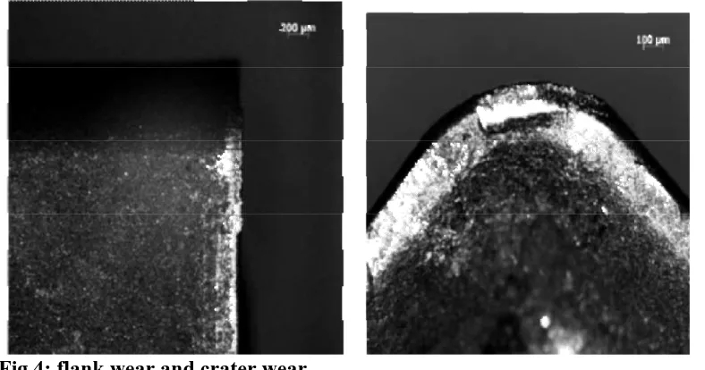
A new cutting edge was used for each run. The resulting tool wear was measured using a Tool makers optical Microscope.

Fig 4: flank wear and crater wear

Process Parameters Table 2:

Code Parameter Level (-1) Level(+1)

A Cutting speed (m/min) 14 40

B Feed (mm/rev) 0.07 0.13

C Depth of cut (mm) 0.5 1.0

Layout of Experiment for RSM Method

(6)

Available online:

https://edupediapublications.org/journals/index.php/IJR/

P a g e |

2574

Table3 Design Layout

Std Order Run

Order Pt Type Blocks

Speed (m/min)

Feed (

mm/rev )

Depth of Cut ( mm )

1 1 1 1 14 0.07 0.50

2 2 1 1 40 0.13 0.50

3 3 1 1 40 0.07 1.00

4 4 1 1 14 0.13 1.00

5 5 0 1 27 0.10 0.75

6 6 0 1 27 0.10 0.75

7 7 1 2 40 0.07 0.50

8 8 1 2 14 0.13 0.50

9 9 1 2 14 0.07 1.00

10 10 1 2 40 0.13 1.00

11 11 0 2 27 0.10 0.75

12 12 0 2 27 0.10 0.75

13 13 -1 3 14 0.10 0.75

14 14 -1 3 40 0.10 0.75

15 15 -1 3 27 0.07 0.75

16 16 -1 3 27 0.13 0.75

17 17 -1 3 27 0.10 0.50

18 18 -1 3 27 0.10 1.00

19 19 0 3 27 0.10 0.75

20 20 0 3 27 0.10 0.75

the most significant parameter affecting surface roughness is nose radius. RESULT AND DISCUSSION

Table 4: observations Std Order _RunOrder speed (m/min) Feed (mm/rev) DoC

(mm) _{Fc (N)}

Ra (µm)

Wear (

mm )

1 1 14 0.07 0.5 1272.1 0.84 0.293

2 2 40 0.13 0.5 621.51 1.78 0.386

3 3 40 0.07 1 733.58 1.84 0.566

4 4 14 0.13 1 1484.3 2.03 0.73

5 5 27 0.1 0.75 1188.7 1.65 0.609

6 6 27 0.1 0.75 1098.4 1.48 0.462

(7)

Available online:

https://edupediapublications.org/journals/index.php/IJR/

P a g e |

2575

8 8 14 0.13 0.5 1234.1 2.06 0.485

9 9 14 0.07 1 1289.6 1.32 0.538

10 10 40 0.13 1 899.2 1.75 1.035

11 11 27 0.1 0.75 1132.4 1.39 0.816

12 12 27 0.1 0.75 1059.7 1.43 0.771

13 13 14 0.1 0.75 1372 1.33 1.068

14 14 40 0.1 0.75 643.83 0.98 0.919

15 15 27 0.07 0.75 1199.6 0.85 0.505

16 16 27 0.13 0.75 1334.2 1.89 0.921

17 17 27 0.1 0.5 1055.6 1.23 0.502

18 18 27 0.1 1 1249.4 1.47 0.981

19 19 27 0.1 0.75 1202.2 1.37 0.811

20 20 27 0.1 0.75 1188.6 1.52 0.787

ANOVA was used to study the effects of different cutting parameters i.e. speed, feed and depth of cut on the responses i.e. cutting force, surface roughness and tool wear.

Table 5.Anova for cutting force

Source DF Seq SS Adj SS Adj MS F P

Blocks 2 48861 13844 6922 3.04 0.104

Regression 9 1161213 1161213 129024 56.67 0 Linear 3 1041130 1041130 347043 152.44 0

speed 1 957496 957496 957496 420.58 0

feed 1 17531 17531 17531 7.7 0.024

doc 1 66104 66104 66104 29.04 0.001

Square 3 95281 95281 31760 13.95 0.002

speed*speed 1 72673 75397 75397 33.12 0

feed*feed 1 21185 22402 22402 9.84 0.014

doc*doc 1 1423 1423 1423 0.63 0.452

Interaction 3 24803 24803 8268 3.63 0.064

speed*feed 1 107 107 107 0.05 0.834

speed*doc 1 881 881 881 0.39 0.551

feed*doc 1 23815 23815 23815 10.46 0.012

Residual

Error 8 18213 18213 2277

Lack-of-Fit 5 11400 11400 2280 1 0.534

Pure Error 3 6812 6812 2271

(8)

Available online:

https://edupediapublications.org/journals/index.php/IJR/

P a g e |

2576

Fig 5. Main Effects Plot of Fc

The main effect plot shows that the cutting force decreases continuously with increase in speed. With the increase in feed, cutting force increases up to certain value and then remains almost constant with further increase in feed. The same curve is seen in case of the variation of cutting force with depth of cut.

Fig6: Interaction plot for Fc

Table 6: ANOVA for surface roughness

Blocks 2 0.25791 0.21394 0.10697 5.96 0.026 Regression 9 2.64496 2.64496 0.29388 16.38 0

Linear 3 2.0359 2.0359 0.67863 37.83 0

speed 1 0.03844 0.03844 0.03844 2.14 0.181

feed 1 1.64025 1.64025 1.64025 91.44 0

(9)

Available online:

https://edupediapublications.org/journals/index.php/IJR/

P a g e |

2577

speed*speed 1 0.01382 0.0473 0.0473 2.64 0.143 feed*feed 1 0.0326 0.01816 0.01816 1.01 0.344 doc*doc 1 0.0104 0.0104 0.0104 0.58 0.468 Interaction 3 0.55224 0.55224 0.18408 10.26 0.004 speed*feed 1 0.09031 0.09031 0.09031 5.03 0.055 speed*doc 1 0.07031 0.07031 0.07031 3.92 0.083 feed*doc 1 0.39161 0.39161 0.39161 21.83 0.002 Residual Error 8 0.1435 0.1435 0.01794

Lack-of-Fit 5 0.117 0.117 0.0234 2.65 0.226 Pure Error 3 0.0265 0.0265 0.00883

Total 19 3.04638

From table 6, we can see that feed, doc and feed * doc have P-value less than 0.05 , hence they are significant. The lack of fit has P-value 0.226, which is desirable.

Here, feed is most significant parameter having smallest P-value among all.

Fig 7: Main effect plots for Ra

(10)

Available online:

https://edupediapublications.org/journals/index.php/IJR/

P a g e |

2578

Fig 8: Interaction plots for Ra Table 8: ANOVA for Tool wear

Blocks 2 0.32743 0.176594 0.088297 10.42 0.006 Regression 9 0.84986 0.849858 0.094429 11.14 0.001 Linear 3 0.64416 0.644159 0.21472 25.33 0 speed 1 0.0004 0.000397 0.000397 0.05 0.834

feed 1 0.22801 0.22801 0.22801 26.9 0.001

doc 1 0.41575 0.415752 0.415752 49.04 0 Square 3 0.14387 0.143867 0.047956 5.66 0.022 speed*speed 1 0.00006 0.048106 0.048106 5.67 0.044 feed*feed 1 0.10635 0.057709 0.057709 6.81 0.031 doc*doc 1 0.03746 0.037456 0.037456 4.42 0.069 Interaction 3 0.06183 0.061833 0.020611 2.43 0.14 speed*feed 1 0.01328 0.013285 0.013285 1.57 0.246 speed*doc 1 0.04205 0.04205 0.04205 4.96 0.057 feed*doc 1 0.0065 0.006498 0.006498 0.77 0.407 Residual Error 8 0.06782 0.067816 0.008477

Lack-of-Fit 5 0.05571 0.055711 0.011142 2.76 0.216 Pure Error 3 0.0121 0.012105 0.004035

(11)

Available online:

https://edupediapublications.org/journals/index.php/IJR/

P a g e |

2579

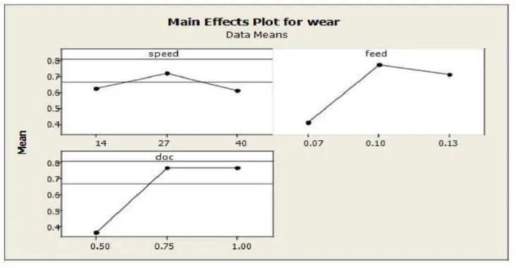
Fig 9: Main effect plot for Flank wear

Graphs show that the tool wear increases with cutting speed up to certain limit and then starts decreasing. Same effect can be seen in case of feed. Wear increases sharply at the starting and then starts decreasing. In case of depth of cut, the flank wear increases at staring and then remains almost constant.

Fig10: interaction plot for Flank wear

Table 9 Estimated Regression Coefficient For Fc

Term Coef SE Coef T P

Constant 1141.69 18.43 61.939 0

Block 1 -9.07 16.06 -0.565 0.588

Block 2 -29.73 16.06 -1.851 0.101

speed -309.43 15.09 -20.508 0

feed 41.87 15.09 2.775 0.024

doc 81.3 15.09 5.389 0.001

speed*speed -167.6 29.12 -5.755 0

(12)

Available online:

https://edupediapublications.org/journals/index.php/IJR/

P a g e |

2580

doc*doc -23.03 29.12 -0.791 0.452

speed*feed -3.65 16.87 -0.217 0.834

speed*doc 10.49 16.87 0.622 0.551

feed*doc 54.56 16.87 3.234 0.012

The regression equation for cutting force is:

S = 47.7137 , PRESS = 220848 R-Sq = 98.52%, R-Sq.(pred) = 82.02% R-Sq(adj) = 96.48 %

Table 10 Estimated regression coefficient for Ra

Constant 1.44712 0.05174 27.969 0

Block 1 0.14837 0.04508 3.291 0.011

Block 2 -0.0283 0.04508 -0.628 0.548

speed -0.062 0.04235 -1.464 0.181

feed 0.405 0.04235 9.562 0

doc 0.189 0.04235 4.462 0.002

speed*speed -0.13275 0.08175 -1.624 0.143

feed*feed 0.08225 0.08175 1.006 0.344

doc*doc 0.06225 0.08175 0.762 0.468

speed*feed -0.10625 0.04735 -2.244 0.055

speed*doc 0.09375 0.04735 1.98 0.083

feed*doc -0.22125 0.04735 -4.672 0.002

S = 0.133933 PRESS = 1.61312 R-Sq = 95.29% R-Sq (pred) = 47.05% R-Sq(adj)

Table 11 Estimated regression coefficient for Tool wear

Constant 0.719438 0.03557 20.227 0

Block 1 -0.124516 0.03099 -4.018 0.004

Block 2 -0.000516 0.03099 -0.017 0.987

speed -0.0063 0.02912 -0.216 0.834

feed 0.151 0.02912 5.186 0.001

doc 0.2039 0.02912 7.003 0

speed*speed 0.133873 0.0562 2.382 0.044

feed*feed -0.146627 0.0562 -2.609 0.031

doc*doc -0.118127 0.0562 -2.102 0.069

(13)

Available online:

https://edupediapublications.org/journals/index.php/IJR/

P a g e |

2581

speed*doc 0.0725 0.03255 2.227 0.057

feed*doc 0.0285 0.03255 0.876 0.407

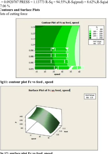
S = 0.0920707 PRESS = 1.13773 R-Sq = 94.55%,R-Sq(pred) = 8.62%,R-Sq(adj) = 87.06 %

Contours and Surface Plots Plots of cutting force

Fig11: contour plot Fc vs feed , speed

Fig 12: surface plot Fc vs feed, speed

(14)

Available online:

https://edupediapublications.org/journals/index.php/IJR/

P a g e |

2582

Fig 13: contour plot Fc vs Doc, speed

Fig14: Surface plot Fc vs doc, speed

(15)

Available online:

https://edupediapublications.org/journals/index.php/IJR/

P a g e |

2583

Fig 15: contour plot Fc vs doc, feed

Fig 16: surface plot Fc vs doc, feed

From this plots we can conclude that cutting force is less for lower value of doc. With the increase in feed cutting force first decrease up to certain value and the

(16)

Available online:

https://edupediapublications.org/journals/index.php/IJR/

P a g e |

2584

Fig 17: contour plot Ra vs feed, speed

Fig 18: surface plot Ra vs feed, speed

(17)

Available online:

https://edupediapublications.org/journals/index.php/IJR/

P a g e |

2585

Fig 19: contour plot Ra vs doc, speed

Fig 20: surface plot Ra vs doc, speed

(18)

Available online:

https://edupediapublications.org/journals/index.php/IJR/

P a g e |

2586

Fig 21: contour plot Ra vs doc , feed

Fig 22: surface plot Ra vs doc, feed

(19)

Available online:

https://edupediapublications.org/journals/index.php/IJR/

P a g e |

2587

Fig 23: contour plot Wear vs feed, speed

(20)

Available online:

https://edupediapublications.org/journals/index.php/IJR/

P a g e |

2588

Fig 25: contour plot wear vs doc, speed

Fig 26: surface plot wear vs doc, speed

(21)

Available online:

https://edupediapublications.org/journals/index.php/IJR/

P a g e |

2589

Fig 27: contour plot wear vs doc, feed

Fig 28: surface plot wear vs doc, feed

Conclusions

(22)

Available online:

https://edupediapublications.org/journals/index.php/IJR/

P a g e |

2590

for tool wear. By optimizing, the optimum values are found to be Speed=40m/min, feed=0.706 mm/rev and doc=0.50mm.

Scope for Future Study

We have conducted the experiment in dry condition using uncoated carbide tool. So, the experiment can be done in wet condition using cutting fluid for better results. In future, applying cutting fluid and taking same work piece –tool combination, the cutting force, surface roughness and tool wear can be analyzed. We have conducted experiment in low speed condition, so by increasing speed the experiment can be done in the future.

Also, MRR, chip reduction coefficient can be added to the output and analyzed taking same combination of tool and work piece and same parameter.

References

1. Dilbag Singh and P.Venkateswara Rao “A surface roughness prediction model for hard turning process”int. J. Adv. Manuf. Technol(2007) 32 : 1115-1124

2. Yang W.H. and Tarng Y.S., (1998), “Design optimization of cutting parameters for turning operations based on Taguchi method,”Journal of Materials Processing Technology, 84(1) pp.112–129.

3. Tugrul Ozel , Tsu-Kong Hsu , Erol Zeren “ Effects of Cutting edge geometry, work piece hardness, feed rate and cutting speed on surface roughness and forces in finish turning of hardened AISI H13 steel”int. J. Adv. Manuf.Technol(2005) 25 : 262-269

4. Neseli S., Yaldiz S. and Turkes E., (2015), “Optimization of tool geometry parameters for turning operations based on the response surface methodology,”Measurement, 44(3), pp. 80-587.

5. Makadia A.J. and Nanavati J.I., (2017), “Optimisation of machining parameters for turning operations based on response surface methodology,” Measurement, 46(4) pp.1521-1529.

6. Bouacha K., Yallese M.A., Mabrouki T. and Rigal J.F., (2010), “Statistical analysis of surface roughness and cutting forces using response surface methodology in hard turning of AISI 52100 bearing steel with CBN tool,”

International Journal of Refractory Metals and Hard Materials, 28(3), pp. 349-361

7. Halim, M.S.B., (2008), “Tool Wear Characterization of Carbide Cutting Tool Insert in a Single Point Turning Operation of AISI D2 Steel,”B.Tech. thesis, Department of Manufacturing Engineering, University Teknikal Malaysia Mekala

8. K. Adarsh Kumar “ Optimisation of surface roughness in face turning operation in machining of EN-8” International Journal of Engineering

Science and emerging technology Vol 2, issue-4, 807-812, July-Aug 2012 9. Srinivas P. and Choudhury S.K., (2004), “Tool wear prediction in turning,”

(23)

Available online:

https://edupediapublications.org/journals/index.php/IJR/

P a g e |

2591

10. Agrawalla, Y, (2014), “Optimization of machining parameters in a turning operation of austenitic stainless steel to minimize surface roughness and tool wear,” B.Tech. thesis, Department of Mechanical Engineering, National Institute of Technology, Rourkela

11. Sharma V.K., Murtaza Q. and Garg S.K., (2010), “Response Surface

Methodology and Taguchi Techniques to Optimization of C.N.C Turning Process,” International Journal of Production Technology, 1(1), pp. 13-31. 12. A.D.Bagawade et all “The cutting conditions on chip area ratio and surface

roughness in hard turning of AISI 52100 steel”international Journal of Enginering research and Technology vol 1 Issue-10 December 2012.

13. Khandey, U., (2009), “Optimization of Surface Roughness, Material

Removal Rate and cutting Tool Flank Wear in Turning Using Extended Taguchi Approach,” MTech thesis, National Institute of Technology, Rourkela 14. Montgomery D.C., Design and Analysis of Experiments, 4th ed., Wiley, New

York, 1997

15. M. Remadna, J.F. Rigal, “Evolution During Time of Tool Wear and Cutting Forces in The Case of Hard Turning With CBN Inserts”, Journal of Materials Processing Technology, vol. 178, pp. 67–75, 2006.

16. Kumar, G., (2013), “Multi Objective Optimization of Cutting and

Geometric parameters in turning operation to Reduce Cutting forces and Surface Roughness,” B.Tech. Thesis, Department of

Mechanical

Engineering, National Institute of Technology, Rourkela 17. N.Chinnasamy. "Prediction and analysis of surface roughness

characteristics of a non-ferrous material using ANN in CNC turning", The International Journal of Advanced Manufacturing Technology, 04/26/2011 18. Mandal, Nilrudra, B. Doloi, and B. Mondal. "Predictive modeling of surface

roughness in high speed machining of AISI 4340 steel using yttria stabilized zirconia toughened alumina turning insert", International Journal of Refractory Metals and Hard Materials, 2013.

19. Chauhan, S. R., and D.Kali "Optimization of Machining Parameters in Turning of Titanium (Grade-5) Alloy Using Response

Surface