A model-based test of the efficacy of a simple rule for predicting adaptive sex allocation

(1)

Scholarship@Western

Electronic Thesis and Dissertation Repository

9-8-2016 12:00 AM

A model-based test of the efficacy of a simple rule for predicting

adaptive sex allocation

Joshua D. Dunn

The University of Western Ontario

Supervisor Dr. Geoff Wild

The University of Western Ontario

Graduate Program in Applied Mathematics

A thesis submitted in partial fulfillment of the requirements for the degree in Master of Science © Joshua D. Dunn 2016

Follow this and additional works at: https://ir.lib.uwo.ca/etd

Part of the Ecology and Evolutionary Biology Commons

Recommended Citation Recommended Citation

Dunn, Joshua D., "A model-based test of the efficacy of a simple rule for predicting adaptive sex allocation" (2016). Electronic Thesis and Dissertation Repository. 4143.

https://ir.lib.uwo.ca/etd/4143

This Dissertation/Thesis is brought to you for free and open access by Scholarship@Western. It has been accepted for inclusion in Electronic Thesis and Dissertation Repository by an authorized administrator of

(2)

Abstract

The division of resources between male and female reproductive function is defined as

sex allocation. The usefulness of simple rules to predict adaptive sex-allocation decisions

has been a contentious topic. Simple rules are difficult to apply when the biological details

of the life cycle are complex, as is the case in many vertebrates. We build a

mathematical-computational model to investigate the usefulness of a simple rule that predicts adaptive

sex-allocation decisions. We find that the simple rule is a better predictor of adaptive sex-sex-allocation

decisions when more features of an organism’s life cycle are assumed to evolve. Even though

the simple rule is a useful heuristic for predicting adaptive sex-allocation decisions, we find that

its usefulness depends critically on the presence or absence of certain sex-specific asymmetries

in the life cycle. We find that magnifying the asymmetries captured by the simple rule improves

the usefulness of the simple rule.

Keywords: sex allocation, sex ratio, Trivers-Willard hypothesis, inclusive fitness, life

his-tory, reproductive value

(3)

The work presented in Chapter 2, which we are currently preparing for submission, is

co-authored by Dr. GeoffWild.

(4)

Acknowlegements

I would like to thank my supervisor, Dr. GeoffWild, for his advice and guidance throughout

most of my academic career. This thesis would not have been possible without the discussions

we have had. I would also like to acknowledge Cody Koykka for helping me figure out how

to put chapter references in this document, among other things. I would like to thank my

examiners, Dr. Lindi Wahl, Dr. Colin Denniston, and Dr. Simon Bonner, for their suggestions

of ways to improve this thesis. I could not have completed this thesis without the love and

support from my parents, David and Janice Dunn. Thank you for always believing in me.

Finally, I appreciate the funding provided by NSERC and the Ontario Graduate Scholarship

program during my Masters degree.

(5)

List of Figures

2.1 Visual representation of the simple allocation rule (SAR) . . . 21

2.2 Verification 1 – Evolution of dispersal . . . 22

2.3 Verification 2 – Evolution of sex allocation . . . 23

2.4 Presentation of results . . . 24

2.5 Fixed dispersal versus evolving dispersal . . . 26

2.6 Adaptive dispersal strategy is unique in most cases . . . 27

2.7 Reducing the asymmetry in sex-specific costs of dispersal improves the predic-tive ability of the SAR . . . 28

2.8 Performance of the SAR becomes invariant to competitive quotients . . . 29

2.9 The SAR is a better predictor of adaptive sex allocation when island sizes are small . . . 31

2.10 Altering island size has a variable effect on adaptive dispersal . . . 31

2.11 The SAR becomes invariant to competitive quotients more quickly when island size is small . . . 32

2.12 Increasing the frequency of good-quality territories does not always have a consistent effect on the predictive ability of the SAR . . . 33

(11)

same sex . . . 35

2.14 The frequency of good-quality breeders has a variable effect on the

perfor-mance of the SAR . . . 36

2.15 Visual representation of which breeder quality causes the simple allocation rule

(SAR) to fail . . . 42

E.1 Reducing the difference sex-specific dispersal costs improves the performance

of the SAR when there is nonzero within-group variation in territory quality . . 100

E.2 Increasing the island size improves the performance of the SAR when there is

nonzero within-group variation in territory quality . . . 100

E.3 The SAR can become invariant to changes in the competitive quotient of the

sex with higher costs of dispersal when there is nonzero within-group variation

in territory quality . . . 101

E.4 The frequency of good-quality territories has a variable effect on the predictive

ability of the SAR when there is nonzero within-group variation in territory

quality . . . 102

(12)

List of Tables

2.1 Summary of mathematical notation used in Chapter 2 . . . 10

(13)

List of Appendices

Appendix A – Inclusive fitness – neighbour-modulated fitness . . . 51

Appendix B – Relatedness . . . 61

Appendix C – Inclusive fitness – biological arguments . . . 66

Appendix D – Code . . . 71

Appendix E – Nonzero relatedness among islandmates of differing quality . . . 92

(14)

Chapter 1 Background and overview

Sex allocation is the division of resources, such as energy and parental care, between male and

female components of Darwinian fitness. This division of resources has a direct effect on the

ratio of males to females in a population, termed the sex ratio. Much theoretical research has

focused on developing simple rules to predict adaptive sex allocation and sex ratios.

Some of the first theoretical work on sex-allocation theory comes from Fisher (1930), who

outlined the situations in which a simple rule of equal allocation to male and female

compo-nents of fitness, modulo rates at which fitness returns are gained, might be considered adaptive

(i.e., there are equal numbers of males and females). To make this argument, Fisher introduced

a concept termed reproductive value, which measures how effective an individual will be at

passing on its genes to others in generations far into the future. He argued that, in diploids

(organisms with two sets of chromosomes), the total reproductive value of all male investment

equals that of all female investment. It follows that investment in the rarer sex will yield a

higher reproductive value payoff. Thus, selection will favour those who invest in the rarer

sex, and assuming returns on investment are realized at the same rate for males and females,

selection will stop when neither sex is rarer (i.e., equal investment). Fisher’s theory of equal

allocation in the sexes (i.e., one should always invest equally in the sexes) is a “simple rule”

(15)

that can be used to predict adaptive sex-allocation decisions.

Fisher’s argument for the advantage of unbiased sex allocation made some tacit

assump-tions. When these assumptions are violated, new simple rules that predict sex-allocation

deci-sions are found. Both of the following theories relax Fisher’s tacit assumption of a well-mixed

population to show that sex ratios can be biased toward the sex that suffers less from

com-petition with same-sex relatives. In some organisms, such as fig wasps in the genus Idarnes, differences in sex-specific morphology are associated with males competing for mates

(Hamil-ton, 1979). When males compete for mates, sex ratios are female biased and the associated

theory is referred to as local mate competition (LMC) (Hamilton, 1967). While studying the

galagid primateGalago crassicaudantus, Clark (1978) noticed that female kin were compet-ing for reproductive resources and sex ratios were biased toward males. This led to the theory

known as local resource competition (LRC), which states that sex ratios are biased toward

males when females compete for reproductive resources. The results given by LMC and LRC

led to a different simple rule that predicts adaptive sex allocation in populations when Fisher’s

well-mixed assumption fails. This simple rule suggested that individuals should invest in the

more dispersive sex, according to Bulmer and Taylor (1980), or invest in the sex more likely

to compete for breeding opportunities on a non-natal territory, according to Wild and Taylor

(2004).

Trivers and Willard (1973) proposed another simple rule that predicts adaptive sex-allocation

decisions by relaxing Fisher’s tacit assumption that same-sex individuals are in the same

con-dition. They assumed that higher quality individuals provide a higher rate-of-return on

in-vestment. Their hypothesis, called the Trivers-Willard hypothesis (TWH), predicted that when

(16)

3

receives a greater benefit for being higher quality. For example, if males or male function

yields higher returns on investment, then breeders in higher condition should invest in males

(or male reproductive function) and breeders in lower condition should invest in females (or

female reproductive function). The investment strategy predicted by the TWH is the result of a

direct incentive for high-quality breeders and a frequency-dependent incentive for low-quality

breeders. Empirical evidence for the TWH was found by Clutton-Brock et al. (1986) while

studying red deer (Cervus elaphus). Hewison and Gaillard (1999) conducted a review of em-pirical studies that tested the TWH in ungulates. They found that while the TWH was able

to correctly predict allocation decisions in some species, such as the red deer (Clutton-Brock

et al., 1986) and the arrui (Ammotragus lervia) (Cassinello, 1996), the TWH was not able to predict allocation decisions in other species, such as the horse (Equus caballus) (Monard et al., 1997). Surprisingly, the conclusions of empirical studies that test the TWH in the same species

may not even agree (i.e., one study may conclude that the TWH was able to predict allocation

decisions and another concludes that the TWH was not able to predict allocation decisions).

This was the case in the reindeer (Rangifer tarandus) (Skogland, 1986; Kojola and Eloranta, 1989). Due to the mixed support of the TWH in vertebrates, the usefulness of this simple rule

when applied to organisms with more complex life histories is currently under debate.

The TWH has generated a lot of interest from biologists. Unfortunately, the TWH has

not been able to correctly predict adaptive sex-allocation decisions in some vertebrate species,

possibly due to non-homogeneity in parental quality accompanied by incomplete mixing. It is

for this reason that Wild and West (2007) sought to investigate the performance of simple rules

based on LMC and TWH when Fisher’s assumptions of homogeneity and complete mixing are

(17)

poor performance of simple rules in their model is underpinned by constrained dispersal. Wild

and Taylor (2004) allowed sex allocation and dispersal to coevolve ( i.e., the joint evolution

of multiple traits in a species) and found that simple rules like equal allocation are recovered.

Specifically, they showed that when there is an asymmetry in sex-specific dispersal rates,

in-dividuals prefer to invest in the sex that disperses more readily. This rule was not recovered

when dispersal rates were fixed. The result in Wild and Taylor (2004) suggests to us that fixing

dispersal may be the reason why simple rules, such as the TWH, cannot be easily applied to

models with more complex life histories, and in turn empirical studies of vertebrates. The first

goal of this work is to determine if the coevolution of sex allocation and dispersal is able to

restore the usefulness of simple rules when applied to vertebrates.

Models inspired by the TWH have assumed zero relatedness between individuals of diff

er-ent quality. This assumption is the result of the chosen population structure: models assume

infinite islands; each island has homogeneous territory quality; individual quality is derived

from territory quality; due to the infinite island structure, individuals on different islands (of

potentially different quality) are unrelated (Leturque and Rousset, 2003; Wild and West, 2007).

However, in nature, when organisms use lek mating – males attempt to attract a female for a

breeding opportunity and then females raise the offspring elsewhere – zero relatedness between

individuals of different quality seems unlikely. For example, lek mating systems are found in

the black grouse (Tetrao tetrix) (Alatalo et al., 1992), and more interestingly in the kakapo (Stringops habroptilus) (Sutherland, 2002) — a species in which the TWH can be applied. The second goal of this work is to address the lack of sex-allocation theory when relatedness is

nonzero between individuals of different quality.

(18)

sex-5

allocation strategy changes the reproductive value of an individual’s genetic lineage, which is

that individual’s inclusive fitness (Taylor, 1990). Inclusive fitness is a measure of how eff

ec-tive an individual is at transmitting its genes, and identical copies of its genes, into the next

generation. Changes in inclusive fitness give us insight into the directional action of selection

for a given trait. We derive changes in inclusive fitness using an excellent modeling heuristic

provided by Taylor and Frank (1996).

Essentially, the method presented in Taylor and Frank (1996) is a perturbation analysis

around the zeroth-order case when no selection is present. They assumed that the expression

of a trait (e.g., sex allocation) is determined by an individual’s genes. Taylor and Frank (1996)

began with a population that has neutral genetic diversity and that had been allowed to reach

an equilibrium. Additionally, they assumed that when the expression of a trait is increased by

an allele, all identical by descent copies of that allele are also able to increase the expression

of that trait. Consequently, increasing the expression of a trait affects reproductive values.

Weighting the new reproductive values by a focal individual’s genetic contribution allows us to

approximate their change in inclusive fitness. The direction of evolution under natural selection

can be determined and an adaptive sex-allocation strategy can be predicted.

InChapter 2, we investigate whether alleviating constraints on the evolution of dispersal

is able to restore the usefulness of simple rules that predict sex-allocation decisions. We

in-vestigate how sex-specific differences in the life history affect the predictive ability of a simple

rule based on the TWH. This is done for the case when all territories on an island are the

same quality, which addresses our first goal. Overall, we find that alleviating constraints on

the evolution of dispersal is able to restore the usefulness of this simple rule. We also find

(19)

Chapter 3reiterates the findings of this thesis and suggests future projects that further

investi-gate how alleviating evolutionary constraints affects the usefulness of simple rules that predict

sex-allocation decisions. In this chapter, we make reference to Appendix E where we present

preliminary results for our second goal. Specifically, we present preliminary results for the

(20)

1.1. References 7

1.1 References

Alatalo, R. V., H¨oglund, J., Lundberg, A., and Sutherland, W. J. (1992). Evolution of black grouse leks: female preferences benefit males in larger leks. Behavioral Ecology, 3(1):53– 59.

Bulmer, M. G. and Taylor, P. D. (1980). Dispersal and the sex ratio. Nature, 284:448–449. Cassinello, J. (1996). High-ranking females bias their investment in favour of male calves in

captiveAmmotragus lervia. Behavioral Ecology and Sociobiology, 38(6):417–424.

Clark, A. B. (1978). Sex ratio and local resource competition in a prosimian primate. Science, 201(4351):163–165.

Clutton-Brock, T. H., Albon, S. D., and Guinness, F. E. (1986). Great expectations: dominance, breeding success and offspring sex ratios in red deer. Animal Behaviour, 34(2):460–471. Fisher, R. A. (1930). The genetical theory of natural selection. Clarendon Press, Oxford. Hamilton, W. D. (1967). Extraordinary sex ratios. Science, 156(3774):477–488.

Hamilton, W. D. (1979). Wingless and fighting males in fig wasps and other insects. In Blum, M. S. and Blum, N. A., editors, Reproductive competition and sexual selection in insects, pages 167–220. Academic Press, New York.

Hewison, A. M. and Gaillard, J.-M. (1999). Successful sons or advantaged daughters? The Trivers–Willard model and sex-biased maternal investment in ungulates. Trends in Ecology

&Evolution, 14(6):229–234.

Kojola, I. and Eloranta, E. (1989). Influences of maternal body weight, age, and parity on sex ratio in semidomesticated reindeer (Rangifer t. tarandus). Evolution, 43(6):1331–1336. Leturque, H. and Rousset, F. (2003). Joint evolution of sex ratio and dispersal: conditions for

higher dispersal rates from good habitats. Evolutionary Ecology, 17(1):67–84.

Monard, A.-M., Duncan, P., Fritz, H., and Feh, C. (1997). Variations in the birth sex ratio and neonatal mortality in a natural herd of horses. Behavioral Ecology and Sociobiology, 41(4):243–249.

Skogland, T. (1986). Sex ratio variation in relation to maternal condition and parental invest-ment in wild reindeerRangifer t. tarandus. Oikos, 46(3):417–419.

Sutherland, W. J. (2002). Conservation biology: science, sex and the kakapo. Nature,

419(6904):265–266.

Taylor, P. D. (1990). Allele-frequency change in a class-structured population. American Naturalist, 135(1):95–106.

(21)

Trivers, R. L. and Willard, D. E. (1973). Natural selection of parental ability to vary the sex ratio of offspring. Science, 179(4068):90–92.

Wild, G. and Taylor, P. D. (2004). Kin selection models for the co-evolution of the sex ratio and sex-specific dispersal. Evolutionary Ecology Research, 6(4):481–502.

(22)

Chapter 2 Coevolution of sex allocation and dispersal

2.1 Introduction

Sexual species face a natural trade-off between investment in male reproductive function on

one hand and female reproductive function on the other. Individuals approach this trade-off

using sex-allocation strategies. Among dioecious species (i.e., species with separate sexes)

sex-allocation strategies determine the sex ratio, either entirely or in part.

Sex allocation has captured the attention of evolutionary biologists because of its obvious

implications for Darwinian fitness and because associated theory makes very clear predictions

(West, 2009). The strongest support for sex-allocation theory has come from organisms that

have simple life histories, often invertebrates (West et al., 2005). For invertebrates in particular,

simple rules are usually sufficient to predict bias in allocation decisions. For example, the

chalcidoid waspPachycrepoideus vindemiaehas been found to bias its allocation towards the more dispersive sex, a rule that is in keeping with theory that invokes competition among

kin (Hamilton, 1967; Nadel and Luck, 1992; Taylor, 1993). Another species, the parasitic

pteromalid waspLariophagus distinguendus, has been found to bias its sex allocation towards the sex that receives a greater benefit from a higher-quality host (Charnov et al., 1981), a rule

(23)

Symbol Definition

N number of territories on an island

pi frequency of islands with quality-iterritories

αi allocation strategy where (i= g,b)

ds,i dispersal strategy where (s= m, f) and (i=g,b)

K number of sons or daughters produced

cs cost of dispersal (s=m, f)

as,i competitive ability (s= m, f) and (i= g,b)

qs the sex-scompetitive quotient and is equal toas,g/as,b

vs,i reproductive value where (s= m, f) and (i= g,b)

Ns,i total competitive pressure on an island where (s= m, f) and (i=g,b)

ks,i probability breeder originated from the quality-ifocal island

Ri relatedness between parent and offspring where (i= g,b)

¯

Ri relatedness between qualityibreeder and offspring on the same island

Table 2.1: Summary of mathematical notation used in Chapter 2

that follows the well known Trivers-Willard hypothesis (TWH) (Trivers and Willard, 1973).

Numerous other examples of invertebrates that support the usefulness of simple rules to predict

sex-allocation decisions can be found (Hoagland, 1978; Charnov, 1979b; Charnov et al., 1981;

Frank, 1985; Werren, 1987; Frank, 1995).

Contrary to support for sex-allocation theory among invertebrate species, the applicability

of simple rules among vertebrate species has been mixed (Clark, 1978; Clutton-Brock et al.,

1986; Hewison and Gaillard, 1999). The difficulty in applying simple sex-allocation rules to

vertebrates, especially those based on the TWH, can be attributed to the relative complexity of

vertebrate life histories. When available theory has tried to cope with the complexities

associ-ated with vertebrates, the predictions generassoci-ated have become less clear. Wild and West (2007)

developed a model that illustrates this point. Their model reflected the complexities commonly

associated with vertebrate life histories, and challenged simple rules of sex allocation by both

allowing for competition among kin and incorporating key features of the TWH. Wild and West

(24)

2.2. Model 11

changed in their model, the simple rules that work so well for invertebrates could fail in drastic

and unexpected ways for vertebrates. This casts further doubt on the usefulness of simple rules

for the study of vertebrate sex allocation, but more theoretical work needs to be done before

we abandon these convenient heuristics.

In this work, we construct a complicated life-history model for the evolution of sex

alloca-tion in order to further explore the usefulness of simple rules in problematic vertebrate species.

Like Wild and West (2007), we challenge simple rules by incorporating competition among

kin and elements of the TWH. Unlike Wild and West (2007), we allow dispersal to evolve

alongside sex allocation. Why do we allow dispersal to evolve? Because it has previously

been shown that when life histories are complex and invoke theory pertaining to competition

among kin, the coevolution or joint evolution of multiple traits in a species restores simple

sex-allocation rules (SAR) (Wild and Taylor, 2004). We find that a SAR based on the TWH can

be useful in understanding model predictions. We also find that improvements in its usefulness

can be due to dispersal evolution. Despite improved success, the SAR can fail and we outline

how it fails in relation to distribution of quality and asymmetries in sex-specific life-history

characteristics. We develop recommendations for the application of this sex-allocation theory

to studies of vertebrates.

2.2 Model

(25)

2.2.1 Preliminaries

We modify previous work (Leturque and Rousset, 2003; Wild and West, 2007) to model the

coevolution of sex allocation and sex-specific natal dispersal. Like many previous authors, we

use a class-structured inclusive-fitness approach based on discrete-time population dynamics

(Taylor and Frank, 1996; Taylor, 1996).

We consider a population made up of diploid dioecious individuals with nonoverlapping

generations. The model population is found in a habitat made up of a very large number of

islands. Each island is subdivided intoN breeding territories, which are either all of good or bad quality. Additionally, we let pi, wherei=g (good),b (bad), denote the fraction of islands

with quality-iterritories (sometimes referred to as a quality-iisland), wherepiremains constant

over time.

For the model, territory quality is important because it defines the quality of a breeder.

Good-quality (resp. bad-quality) breeders produce good-quality (resp. bad-quality) offspring.

However, offspring quality is only temporary. An offspring that establishes itself as a breeder

takes on the quality of its newly found territory. For the sake of brevity, we use the terms

quality-ibreeder, quality-ibreeding pair (a breeding female and her mate), and quality-ioff -spring, wherei=g,b, as we develop the model below.

2.2.2 Life cycle

The life cycle consists of a series of life-history events (or “stages”) that occur in the following

(26)

2.2. Model 13

Birth

Each breeding pair producesKsons andK daughters, whereK is very large.

Parental care

A quality-ibreeding female has a fixed amount of some resource that they must entirely devote to offspring. She allocates the fractionαi to sons and 1−αi to daughters, leaving them with

Kαi quality-isons and K(1−αi) quality-idaughters. We constrain the allocation behaviour to

be biologically relevant (i.e., 0 < αi < 1). We assume that allocation decisions are controlled

by the genotype of the female member of the breeding pair (i.e., we assume maternal control).

We also assume that, after investment, all breeding pairs in the population die. At this point,

only offspring remain.

Dispersal

Quality-ioffspring disperse independently, with probabilityds,i, wheres=m (male), f (female).

We constrain dispersal to be biologically relevant (i.e., 0 <ds,i <1). We assume that dispersal

is determined by the gynotype of the offspring itself (i.e., under offspring control). We also

assume that dispersal is costly. The cost associated with dispersal for males and females iscm

and cf, respectively. This means that only fraction 1−cs of sex-s dispersers survive to the

next stage in the life history. Offspring who do not disperse do not pay a cost and survive to

the next stage in the life history with probability equal to one. Offspring that disperse do so

independently and compete for territories on an island, which is chosen uniformly at random

from the collection of all islands in the population. Consequently, offspring cannot choose the

(27)

compete for territories on their natal island.

Male-male competition

Following the dispersal stage, male offspring compete for mates. The competitive ability of a

good-quality male offspring isam,g and the competitive ability of a bad-quality male offspring

isam,b, and we often focus on the ratioqm =am,g/am,b ≥1, which we call the male competition

quotient (MCQ). The total amount of male competitive effort on a quality-i island is denoted byNm,i and is calculated in Appendix A. Competition itself is modelled as a weighted lottery

withqmas weights.

The weighted lottery works as follows. Each male offspring competing for a given

terri-tory has a number of “tickets” that is directly proportional to its competitive ability, am,i. The

tickets of all male offspring competing on an island are collected, and tickets are then selected

uniformly at random with replacement untilN are chosen. Male offspring whose tickets have been chosen, win a breeding opportunity, and those whose tickets have not been chosen die.

Female-female competition

Female offspring compete for breeding territories. The competitive ability of a good-quality

female offspring isaf,gand the competitive ability of a bad-quality female offspring isaf,b, and

we often focus on the ratioqf = af,g/af,b ≥ 1, which we call the female competition quotient

(FCQ). The total amount of female competitive effort on a quality-iisland is denoted by Nf,n

and is calculated in Appendix A. Competition itself is modelled as a weighted lottery (see

(28)

2.2. Model 15

We allow forqmandqf to be different, and so we allow for sex-specific differences in returns

on parental allocation. This is a key difference between ours and previous work (Leturque and

Rousset, 2003). We also do not restrict ourselves to the assumption that males always receive

a greater benefit for being a good-quality offspring. This means that we consider bothqm>qf

andqm <qf, unlike Wild and West (2007).

2.2.3 Inclusive fitness overview

We describe the evolutionary consequences of the model life history using an inclusive-fitness

approach (Hamilton, 1964; Taylor and Frank, 1996; Taylor, 1996). Inclusive fitness can be

defined in terms of reproductive value, in other words, an individual’s contribution to the gene

pool in the very distant future (Fisher, 1930). Specifically, the inclusive fitness of a given

individual is its genetic stake in the reproductive value of its contemporaries; it can be written

as a weighted sum of reproductive values, where weights are coefficients of genetic relatedness

(see Michod and Hamilton, 1980).

In this work, we do not study inclusive fitness per se, rather we studychangesin inclusive fitness. Moreover, for our purposes it will be convenient to split changes in inclusive fitness into

two components: direct and indirect. The former represents gains achieved through production

of immediate descendants and personal survival. The latter represents gains achieved through

(29)

2.2.4 Evolution of sex allocation

To apply the inclusive-fitness approach to the evolution of sex allocation we fix attention on

a quality-i breeding female. We assume that this mutant individual, and only this mutant in-dividual, increases its allocation strategy, αi, by a very small amount (Taylor, 1989). If the

inclusive-fitness change is positive, the mutation is beneficial and becomes the new wildtype

behaviour. We assume that changes in inclusive fitness are independent of the frequency of

in-dividuals using the mutant behaviour in the population. Further, we assume that two mutations

are not occurring simultaneously, which allows us to treat this process as a first-order

pertur-bation analysis. In Appendix A, we use a modeling technique developed by Taylor and Frank

(1996) to show the resulting changes in the inclusive fitness of the focal individual, holding all

other sex allocation and dispersal traits in the population fixed, can be expressed as

∆W_iα∝X

j

(1−dm,i)am,i

Nm,i

Nvm,jRi−

(1−df,i)af,i

Nf,i

Nvf,jRi | {z }

sex-allocation term A

+X

j

pj

dm,i(1−cm)am,i

Nm,j

Nvm,jRi−pj

df,i(1−cf)af,i

Nf,j

Nvf,jRi | {z }

sex-allocation term B

−km,i

(1−dm,i)am,i

Nm,i

Nvm,iR¯i | {z }

sex-allocation term C

+kf,i

(1−df,i)af,i

Nf,i

Nvf,iR¯i | {z }

sex-allocation term D

                                                   , (2.1)

wherevs,i is the individual reproductive value of a sex-squality-ibreeder,ks,i is the probability

a sex-squality-ioffspring would have won a breeding opportunity (s=m) or territory (s= f),

Riis the relatedness between a quality-ibreeder and its own offspring, and ¯Riis the relatedness

(30)

2.2. Model 17

we provide a complete biological interpretation of the above equation.

Recall that the inclusive-fitness change in equation (2.1) is derived by assuming a

mu-tant quality-i breeding female invests slightly more resources into sons, and in turn, invests slightly fewer resources into daughters. As a result, more sons and fewer daughters of the

mutant quality-i breeding female are surviving the parental care stage of the life cycle, com-pared to the wildtype quality-ibreeding female. The inclusive-fitness change in equation (2.1) can be broken down into four terms. The first term (sex-allocation term A) is the sum of

direct fitness gains through non-dispersing sons on one hand, and direct

inclusive-fitness losses through non-dispersing daughters. The second term (sex-allocation term B) is

the difference of direct inclusive-fitness gains through dispersing sons on one hand, and direct

inclusive-fitness losses through dispersing daughters on the other. Sex-allocation terms A and

B show that the focal breeding female faces a trade offbetween the production of sons and the

production of daughters. The third term (sex-allocation term C) represents indirect

inclusive-fitness losses due to increased competition for mates that comes from non-dispersing sons. The

fourth term (sex-allocation term D) represents indirect inclusive-fitness gains due to decreased

competition for breeding territories that comes from fewer non-dispersing daughters.

Sex allocation terms A through D, together, describe the overall inclusive-fitness change of

a quality-ibreeding female slightly increasing its allocation strategy. When ∆W_iα is positive (resp. negative), it is beneficial for the breeding female to slightly increase (resp. decrease) its

(31)

2.2.5 Evolution of dispersal

To apply the inclusive-fitness approach to the evolution of dispersal we fix attention on a

sex-s quality-i offspring. We assume that this individual, and only this individual, increases its probability of dispersal,ds,i, by a very small amount (Taylor, 1989). In Appendix A, we use a

modeling heuristic developed by Taylor and Frank (1996) to show the resulting changes in the

inclusive fitness of the focal individual, holding all other sex allocation and dispersal traits in

the population fixed, can be expressed as

∆Wsd,i ∝ −

X

j

1

Nm,i

NRivs,j | {z }

dispersal term A

+(1−cs)

X

j

pj

1

Ns,j

NRivs,j | {z }

dispersal term B

+ks,i

1

Ns,i

NR¯ivs,i | {z } dispersal term C

                                                     . (2.2)

In Appendix C, we provide a complete biological interpretation of the above equation.

Recall that the inclusive-fitness change in equation (2.2) is derived by assuming a

mu-tant sex-s quality-i offspring disperse slightly more frequently. As a result, this offspring is more likely to compete on a non-natal territory than a wildtype offspring. The inclusive-fitness

change for dispersal in equation (2.2) can be broken down into three terms. The first term

(32)

2.3. Method of analysis 19

competition for mates or decreased competition for breeding territories whens= mands= f, respectively.

Dispersal terms A through C, together, describe the overall inclusive-fitness change of a

sex-s quality-i offspring island that slightly increases its dispersal strategy. When ∆Wd s,i is

positive (resp. negative), it is beneficial for the offspring to slightly increase (resp. decrease)

its current dispersal strategy.

2.3 Method of analysis

2.3.1 Evolutionary stability and numerical procedure

We are interested in finding adaptive sex-allocation and dispersal traits, ˆαiand ˆds,ifor all sand

i. To find the adaptive traits, we use equations (2.1) and (2.2) derived above. Recall that these equations tell us the direction of selection for sex-allocation and dispersal traits, respectively.

When∆W_iα> 0 (resp. <0), selection favours sex-allocation strategies that invest slightly more (resp. fewer) resources in male offspring than the current strategy. Similarly, if∆Wd_s_,_i > 0 (resp.

< 0), selection favours strategies that result in more (resp. less) frequent dispersal. Due to

the complexity of this model we determine ˆαi and ˆds,iusing a numerical procedure. In general,

we begin our procedure by proposing a set of strategies, αi and ds,i. Based on the proposal

we determine the signs of inclusive-fitness changes described by (2.1) and (2.2). Then we

update our proposal according to sign of the associate inclusive-fitness expression. If∆W_iα >0 (resp. < 0) we increase (resp. decrease) αi by a small amount that is proportional to the

(33)

that is proportional to the magnitude of ∆W_sd_,_i. We continue to update until the change in the proposal is sufficiently small. We check multiple initial proposals to see if there are multiple

adaptive strategies (there were none). The code that implements this algorithm can be found in

Appendix D.

2.3.2 The simple allocation rule (SAR)

We test the predictive strength of a version of the TWH, which we henceforth refer to as the

SAR. The SAR will be said to “work” or is a “strong/good predictor of allocation decisions”

when good-quality breeders invest more resources in sons and bad-quality breeders invest more

in daughters when sons receive a greater benefit for being a good-quality offspring (qm > qf).

The SAR also works when good-quality breeders invest more resources in daughters and

bad-quality breeders invest more in sons when daughters receive a greater benefit for being a

good-quality offspring (qm >qf). Mathematically, the SAR works when

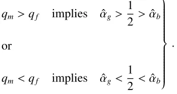
qm >qf implies αˆg >

1 2 > αˆb

or

qm <qf implies αˆg <

1 2 < αˆb

                          

.

Conversely, the SAR will be said to “fail” or is a “poor/bad predictor of allocation decisions”

when the above conditions do not hold. A visual representation of the SAR can be found in

Figure 2.15.

We focus on a SAR based on the TWH rather than a SAR based on LRC because parent

(34)

2.3. Method of analysis 21

Figure 2.1: Visual representation of the simple allocation rule. When good-quality sons are the better intrasexual competitor (occurs whenqm> qf), good-quality breeders should invest more

in sons (αg > 1₂) and bad-quality breeders should invest more in daughters (αb < 1₂). When

good-quality daughters are the better intrasexual competitor (occurs when qm < qf),

good-quality breeders should invest more in daughters (αg < 1₂) and bad-quality breeders should

invest more in sons (αb > 1₂).

require information about migration patterns and genetic relatedness, and these are unlikely to

be as easy to uncover as measures of quality (e.g., size or weight). Essentially, we focus on the

TWH because the associated variables are likely to be easier to measure.

2.3.3 Previous results as special cases

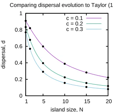
To validate our numerical procedure we test it with several well-known special cases. First, we

compare to the work in Taylor (1988). Here, we consider a homogeneous population (pg = 1

and pb = 0), we allow for no sex-specific competitive differences (qm = qf = 1), and no

sex-specific costs of dispersal (cm = cf). Following Taylor (1988), sex allocation is constrained to

be unbiased (αg = 0.5) and dispersal rate is constrained to be the same for male and female

(35)

sizesN =1, ...,20 (Figure 2.2).

A second comparison is to the work in Charnov (1979a) and Bull (1981). Here, we consider

a population that consists of islands with only one good or bad territory (N =1). We constrain the model so that dispersal is complete (ds,i = 1) and cost-free for both male and female

offspring (cm = cf = 0). As before, we find that our numerical procedure recovers the results

of Charnov (1979a) and Bull (1981) (Figure 2.3).

A third comparison is to the work in Wild and West (2007), described in the introduction.

As in the second comparison, the population consists of islands with only one good or bad

quality territory (N = 1). Male-offspring dispersal among these islands is constrained to be complete (dm,i = 1). By contrast, female dispersal is constrained, and though it may be

in-complete, is independent of island/territory quality (df,i = df for all iandn). All dispersal is

cost-free (cm = cf = 0). Our numerical procedure recovers tabulated results in Wild and West

(2007).

dispersal, d

island size, N

Comparing dispersal evolution to Taylor (1988)

c = 0.1 c = 0.2 c = 0.3

0 0.2 0.4 0.6 0.8 1

1 5 10 15 20

Figure 2.2: We find agreement between the predictions in Taylor (1988) (solid coloured lines) and those generated by our model (black dots). To make this comparison we setpg= 1,pb = 0,

(36)

2.4. Results 23

Comparing sex-allocation evolution to Charnov (1979a) and Bull (1981)

sex allocation,

α

good- to bad-quality ratio, p_g/p_b p_g/p_b < q_f < q_m

0 0.2 0.4 0.6 0.8 1

0 0.5 1 1.5 2

sex allocation,

α

good- to bad-quality ratio, p_g/p_b q_f < p_g/p_b < q_m

good-quality bad-quality

0 0.2 0.4 0.6 0.8 1

2 2.5 3 3.5 4

sex allocation,

α

good- to bad-quality ratio, p_g/p_b q_f < q_m < p_g/p_b

0 0.2 0.4 0.6 0.8 1

4 6 8 10 12 14 16 18 20

Figure 2.3: We find the agreement between the predictions in Charnov (1979a) and Bull (1981) (solid lines) and those generated by our model (red and blue dots). The red dots represent the sex-allocation strategy of good-quality breeders and blue dots represent the sex-allocation strategy of bad-quality breeders. We denote the frequency of good-quality breeders and the frequency of bad-quality breeders as pg and pb, respectively. For this figure we set N = 1,

ds,i = 1 for allsandi,cm=cf =0,qm= 4, andqf =2.

2.4 Results

2.4.1 Setting the stage

This section is used to explain how we will present results in this work. Rather than presenting

the stable strategies themselves, we use graphical tools to evaluate the performance of the SAR.

As the cartoon in Figure 2.4 shows, we divideqm,qf-space into regions where the SAR works

and where it fails. We then propose a rationale for the observed changes in these regions, given

concomitant changes in parameters, and in the absence of analytical solutions of the model.

2.4.2 Dispersal evolution improves the performance of the SAR

In this subsection, we compare the predictive strength of our SAR when dispersal is allowed

(37)

female competitive quotient, q

f

male competitive quotient, q_m

Figure guide

1 2 3 4 5 6 7 8 9

Simple rule fails

Simple rule works

Figure 2.4: This cartoon shows how results will be presented in this work. Blue regions repre-sent areas of parameter space where the SAR works and red regions reprerepre-sent areas of param-eter space where the SAR fails. The central dashed gray line separates two distinct regions of parameter space. Below the gray dashed line the MCQ is greater than the FCQ (qm > qf) and

(38)

2.4. Results 25

we use equations (2.1) and (2.2), whereas when dispersal is not allowed to evolve we only use

equation (2.1) with fixed values of dispersal. For this comparison we set the costs associated

with dispersal to be the same for males and females (cm = cf). Under these conditions, when

dispersal is allowed to evolve we find that the SAR always works (Figure 2.5c). We also find

that the dispersal rate for a sex-squality-ioffspring is unique in most cases (Figure 2.6). When dispersal is not allowed to evolve, we find that the SAR can fail (Figure 2.5a and b). Granted,

results presented in Figure 2.5 assume that dispersal is sex-specific, but not conditioned on

offspring quality (dm =dm,g =dm,banddf =df,g = df,bfollowing Wild and West (2007)). This

assumption could exacerbate the failure of the SAR when dispersal is not allowed to evolve.

However, because the SAR always works when dispersal isallowed to evolve, any failure in the SAR when dispersalis notallowed to evolve represents poorer performance.

Why does constraining dispersal evolution reduce the performance of the SAR? Simply

put, when dispersal is not allowed to evolve there are fewer “evolutionary degrees of freedom”.

In this case, sex allocation alone has to balance competing inclusive-fitness interests, which

results in compromises that would not be seen when sex allocation and dispersal coevolve.

Based on this result, we suggest that the concerns raised by Wild and West (2007) regarding

the application of verbal sex-allocation theory (simple rules) may be overstated.

2.4.3 Reducing sex-specific di

ff

erences in dispersal cost improves the

per-formance of the SAR

As mentioned in the preceding subsection, the SAR always works when dispersal is allowed to

(39)

Symmetric sex-specific costs of dispersal (c_m = c_f)

f

male competitive quotient, q_m (a) dispersal is fixed (d_m > d_f)

1 2 3 4 5 6 7 8 9 10

1 2 3 4 5 6 7 8 9 10 female competitive quotient, q

f

male competitive quotient, q_m (b) dispersal is fixed (d_m < d_f)

1 2 3 4 5 6 7 8 9 10

f

male competitive quotient, q_m (c) dispersal evolves

1 2 3 4 5 6 7 8 9 10

Figure 2.5: Allowing dispersal to evolve makes the predictive strength of the SAR better when the sex-specific costs of dispersal are equal (cm = cf). For all panels we set the pg = 0.6,

N = 10, and cm = cf = 0.2. (a) In this panel, dispersal is fixed and we assume that male

offspring disperse at a higher rate compared to female offspring (dm = dm,g = dm,b = 1.0 and

df = df,g = df,b = 0.5). The SAR fails for a large region of parameter space. (b) In this

panel, dispersal is fixed and we assume that male offspring disperse at a lower rate compared to female offspring (dm = dm,g = dm,b = 0.5 anddf = df,g = df,b = 1.0). Again, the SAR fails

(40)

2.4. Results 27

f

male competitive quotient, q_m (a) the success of the simple rule

1 2 3 4 5 6 7 8 9

dispersal rate, d

s,i

male competitive quotient, q_m (b) sex-specific dispersal rates

d_m,g d_f,g dm,b d_f,b

0 0.2 0.4 0.6 0.8 1

1 2 3 4 5 6 7 8 9

Figure 2.6: When the costs of dispersal are the same for males and females (cm = cf) and

sex allocation and sex-specific dispersal coevolve, dispersal rates for each sex and quality of offspring are unique in most cases. In this plot, we set pg = 0.7, cm = cf = 0.2, andN = 10.

(a) The SAR always works. We look at the dispersal rates whenqf = 5, which is marked by

the solid black horizontal line. (b) This panel shows the dispersal rates for each sex and quality of offspring. The dispersal rate of good-quality males (dm,g) is in purple, the dispersal rate of

good-quality females (df,g) is in green, the dispersal rate of bad-quality males (dm,b) is in blue,

and the dispersal rate of bad-quality females (df,b) is in yellow. The vertical gray dashed line

represents whenqm =qf =5.

sex-specific costs of dispersal (i.e.,cm, cf), the SAR can fail, even when sex-specific dispersal

and sex allocation coevolve. We find that as the asymmetry in sex-specific costs of dispersal

is increased, there is a decline in the performance of the SAR (Figure 2.7). Conversely, if

we reduce the asymmetry in the sex-specific costs of dispersal, the performance of the SAR

improves. This result is due to the fact that sex allocation reflects sex-specific asymmetries

in the life history. By reducing other asymmetries, such as those stemming from the costs of

dispersal, we bring asymmetries due to competitive advantage into sharper focus; this drives

(41)

f

male competitive quotient, q_m (a) cm = 0.3 and cf = 0.0

1 2 3 4 5 6 7 8 9 10

f

male competitive quotient, q_m (b) cm = 0.3 and cf = 0.1

1 2 3 4 5 6 7 8 9 10

f

male competitive quotient, q_m (c) overlaying panels (a) and (b)

1 2 3 4 5 6 7 8 9 10

Figure 2.7: Reducing the asymmetry in the sex-specific costs of dispersal improves the perfor-mance of the SAR. In this figure, sex-specific dispersal is able to evolve and we set pg = 0.7,

N = 10, andcm = 0.3. (a) This panel shows where the SAR fails when there is an asymmetry

in the sex-specific costs of dispersal. We set cf = 0.0. (b) This panel shows where the SAR

fails when we decrease the asymmetry in the sex-specific costs of dispersal compared to those in panel a). (c) This panel overlays the outline of the failure region from panels a) and b). The purple curves correspond to the initial asymmetry and the green curves correspond to when the asymmetry is reduced.

2.4.4 The predictive ability of the SAR can become invariant to

competi-tive quotients

In this subsection, we show that the predictive strength of the SAR is affected by constraints on

behaviour. We constrain dispersal and sex allocation so that the values are biologically relevant

(i.e., 0 < dˆs,i < 1 and 0 < αˆi < 1). By bounding behaviour to biologically relevant ranges,

the success or failure of the SAR can depend entirely onqs0 whenc_s > c_s0, q_s > q_s0, andq_sis

sufficiently large. In other words, the point of failure of the SAR will occur at the same value

ofqs0 for large ranges ofq_s(Figure 2.8). Whenc_s>c_s0 andq_sis sufficiently large, bad-quality

(42)

2.4. Results 29

f

5 10 15 20 25 30 35

Figure 2.8: The success or failure of the SAR becomes invariant to the competitive quotient of the sex with a higher dispersal cost. This plot depicts the case where the performance of the SAR becomes invariant to the MCQ (qm) since we set cm > cf. Below the center dashed line

the SAR always fails at the same value ofqf whenqmis sufficiently large. To create this figure

we set pg =0.7,cm=0.3,cf = 0.0, andN =10.

and good-quality offspring to use strategies that are invariant to changes in qs. Essentially,

when sufficiently large, the competitive quotient of the sex with a higher cost of dispersal does

not affect the success or failure of the SAR.

2.4.5 Increasing the di

ff

erences in sex-specific competitive quotients does

not reduce the performance of the SAR

As expected, when sex-s offspring have a higher competitive quotient than sex-s0 _off_spring (qs > qs0), increasing q_s never makes the SAR a worse predictor of adaptive sex-allocation

(43)

asymmetries in the life history of the sexes. This allows us to effectively ignore other

compo-nents of the life history when constructing verbal arguments that predict allocation decisions.

Refer to bottom right and top left corners of Figure 2.7. As mentioned in the above section, the

performance of the SAR can become invariant to the competitive quotient of the sex with the

higher cost of dispersal. When invariant, further increasing qs will have no affect on the

per-formance of the SAR (bottom right corner of Figure 2.8). Thus, with all else being equal and

whenqs>qs0, increasingq_smay cause the SAR to work where it otherwise would have failed,

but increasingqswill never cause the SAR to fail where it otherwise would have worked.

2.4.6 Increasing island size has a variable e

ff

ect on the performance of

the SAR

The effect of changing the island size has a potential relationship with sex-specific costs of

dispersal. As we reduce the island size,N, with asymmetric costs of dispersal, the performance of the SAR increases (Figure 2.9). We propose that this stems from the fact that dispersal has

the benefit of reducing competition among relatives. To be clear, as island size is reduced, a

series of events occurs: the relatedness among kin increases, which increases indirect

inclusive-fitness benefits of dispersal and essentially removes existing asymmetries in the sex-specific

costs of dispersal. This rationale is somewhat speculative because dispersal could evolve to

higher levels with decreasing island size, thus modifying the realized sex-specific costs of

dispersal. Additional investigations however, indicate that any reduction in dispersal rates are

not universal (Figure 2.10).

(44)

2.4. Results 31

f

male competitive quotient, qm

(a) N = 10

1 2 3 4 5 6 7 8 9 10

f

(b) N = 20

1 2 3 4 5 6 7 8 9 10

f

(c) overlaying panels (a) and (b)

1 2 3 4 5 6 7 8 9 10

Figure 2.9: Increasing the island size decreases the performance of the SAR. In this figure, sex-specific dispersal is able to evolve and we set pg = 0.7, N = 10,cm = 0.3, andcf = 0.1.

(a) This panel shows where the SAR fails whenN =10. (b) This panel shows where the SAR fails whenN = 20. (c) This panels overlays the outline of the failure region from panels a) and b). The purple curves correspond toN =10 and the green curves correspond toN =20.

f

(a) p_g = 0.3

1 2 3 4 5 6 7 8 9

f

(b) p_g = 0.7

N = 10 N = 20

1 2 3 4 5 6 7 8 9

Figure 2.10: When we increase the size of an island dispersal does not always decrease. The orange points denote areas of parameter space where at least one class of offspring increases

their dispersal rate when we increasing island size from N = 10 to N = 20. The region

outlined by the green curves is where the SAR fails whenN = 10. The region outlined by the purple curves is where the SAR fails when N = 20. Throughout this panel we setcm = 0.3

and cf = 0.1. (a) The frequency of good-quality islands is pg = 0.3. (b) The frequency of

(45)

f

N = 5 N = 10 N = 20

2 4 6 8 10 12 14 16 18 20

Figure 2.11: Smaller island sizes cause the performance of the SAR to become invariant to the competitive quotient of the sex with higher dispersal costs more quickly. In this plot the SAR becomes invariant to the MCQ, qm, sincecm > cf. In this plot we set pg = 0.7,cm = 0.3, and

cf = 0.1. We also varied island size through the values N = 5,10,20. Recall that the region

between the curves of the same color is where the SAR fails. If the top curve is not present for a given color or a curve of a given color disappears, the diagonal dashed line acts as the top curve.

quotient of the sex with higher dispersal costs. Smaller island sizes cause the SAR to become

invariant to lower valuesqs whencs > cs0 (Figure 2.11). We argue that bad-quality breeders

and bad-quality offspring are reaching the bounds on the biologically relevant ranges of sex

(46)

2.4. Results 33

inconsistent effect

of increasing p_g

f

p_g = 0.2

p_g = 0.3

p_g = 0.4

p_g = 0.5

p_g = 0.6

p_g = 0.7

5 10 15 20 25 30 35

Figure 2.12: Increasing the frequency of good-quality territories does not always have a consis-tent effect on the predictive ability of the SAR when competitive quotients are at intermediate values. In this plot we set cm = 0.3, cf = 0.1, and N = 10. We vary the frequency of

good-quality territories in for the valuespg =0.2,0.3,0.4,0.5,0.6,0.7, and the associated line colors

can be found in the legend.

2.4.7 Distribution of quality critically influences the performance of the

SAR

As we have mentioned, if costs of dispersal are symmetric the SAR always works. However,

if the costs of dispersal are asymmetric we find that the SAR can fail in a way that depends

on the distribution of breeder quality. When competitive quotients are at intermediate values,

increasing or decreasing the frequency of good-quality islands does not affect the predictive

ability of the SAR in a consistent fashion (Figure 2.12). The results presented below only hold

when competitive quotients are very small or very large. To explain our findings as we change

distribution of breeder quality we divide our presentation into two cases.

(47)

good-quality breeders to invest more in sex-soffspring and bad-quality breeders to invest more in sex-s0 _off_{spring. While the bad-quality breeders always invest according to the SAR,} good-quality breeders do not (Figure 2.13). In short, whether the SARs fails or not depends on what

good-quality breeders do.

Following comments in the previous section, we know that, when cs > cs0 andq_s > q_s0,

good-quality breeders may not invest according to the SAR because high relative costs of

sex-s dispersal act to diminish competitive gains made by sex-s offspring. As the distribution of breeder quality shifts towards greater frequencies of good-quality breeders, competition

pools contain greater numbers of good-quality offspring. In turn, greater numbers of

good-quality sex-s offspring implies a reduction in their realized competitive advantage, pushing good-quality breeders towards (or further towards) investment strategies contrary to the SAR.

Indeed, as pg is increased in the first case, the SAR becomes a worse predictor of allocation

decisions, which can be seen Figure 2.14.

Next, we look at the case when cs > cs0 and q_s < q_s0. From the SAR we should always

expect good-quality breeders to invest more in sex-s0 offspring and bad-quality breeders to invest more in sex-soffspring. While the good-quality breeders always invest according to the SAR in this case, bad-quality breeders do not (Figure 2.13). Now, whether the SAR fails or not

depends on what bad-quality breeders do.

In this case, bad-quality breeders may not invest according to the SAR because high

rel-ative costs of sex-s dispersal act to diminish competitive gains made by sex-s offspring. As the distribution of breeder quality shifts towards greater frequencies of good-quality breeders,

competition pools contain smaller numbers of bad-quality offspring. In turn, smaller numbers

(48)

bad-2.4. Results 35

f

(a) the success of the simple rule

1 2 3 4 5 6 7 8 9 10

sex-allocation strategy,

αi

(b) cross section of a) at q_f = 5.5

good quality bad quality 0

0.2 0.4 0.6 0.8 1

1 2 3 4 5 6 7 8 9 10

Figure 2.13: When the SAR fails only one quality of breeder allocates in a way that is not predicted. In this plot we set pg = 0.7, cm = 0.3, and cf = 0.1. (a) This panel shows where

the SAR works and fails using a familiar plot. (b) Here we take a cross section of panel a) at the horizontal solid black line (qf = 5.5). The purple curve in panel b) represents the

sex-allocation strategy of good-quality breeders and the dark blue line represents the sex-sex-allocation strategy of bad-quality breeders. The horizontal gray short-dash line marks offthe strategy of equal allocation. The vertical gray long-dash line marks offwhenqm =qf =5.5. To the left of

this lineqm< qf and to the right of this lineqm> qf. We can see that to the left of the vertical

gray long-dash line, good-quality breeders always invest according to the SAR, and to the right of the vertical gray long-dash line, bad-quality breeders always invest according to the SAR. The success or failure of the SAR is always a result of only one quality of breeder allocating incorrectly.

quality breeders towards investment strategies that agree with the SAR. As pg is increased in

the second case, the SAR becomes a better prediction of allocation decisions, which can be

(49)

f

(a) p_g = 0.3

1 2 3 4 5 6 7 8 9 10

f

(b) p_g = 0.7

1 2 3 4 5 6 7 8 9 10

f

(c) overlaying panels (a) and (b)

1 2 3 4 5 6 7 8 9 10

frequency 0

1

goodbad frequency 0

1

goodbad frequency 0

1

goodbad

Figure 2.14: Increasing the frequency of good-quality breeders has a variable effect on the performance of the SAR. In this figure, sex-specific dispersal is able to evolve and we set

pg = 0.7, N = 10, cm = 0.3, and cf = 0.1. The nested plot (top left in each panel) shows

the frequency of good- and bad-quality breeders in the population. (a) This panel shows where the SAR fails when pg = 0.3. (b) This panel shows where the SAR fails when pg = 0.7. (c)

This panel overlays the outline of the failure region from panels a) and b). The purple curves correspond to pg = 0.3 and the green curves correspond to pg = 0.7. Whenqm > qf (below

the dashed line), increasing pgreduces the performance of the SAR. Whenqm<qf (above the

(50)

2.5. Discussion 37

2.5 Discussion

2.5.1 Recapitulation

In this work, we build an inclusive-fitness based model for the coevolution of sex allocation

and sex-specific dispersal with extensive differences in the life history of the sexes. We use the

model to test the predictive strength of a SAR for predicting adaptive sex-allocation decisions.

The rule, itself, is a version of the TWH. Overall, we find that the success or failure of the SAR

boils down to sex-specific differences in the life history.

The success of the SAR improves as sex-specific differences in competitive ability come to

overshadow all others. How can we make sex-specific difference in competitive ability

over-shadow all others? We can do it in two basic ways. The first is by increasing the competitive

ability of one (and only one) sex. The second is by reducing the other sex-specific differences

in life history.

Improvement in the first category is seen as we increase the advantage of a good-quality

individual of one (and only one) sex relative to a same-sex competitor of lower quality (§2.4.5).

It is also seen when we increase the advantage of a good-quality individual of one (and only

one) sex relative to an average same-sex competitor (§2.4.7).

Improvement in the second category is seen as we decrease the differences in sex-specific

cost of dispersal directly or by changes to the mitigating factors, such as social group size

(§2.4.3). We argue that the effect of dispersal evolution also falls into the second category.

When dispersal is fixed, sex allocation has to reflect all sorts of sex-specific differences in life

A model-based test of the efficacy of a simple rule for predicting adaptive sex allocation

Scholarship@Western

Scholarship@Western

A model-based test of the efficacy of a simple rule for predicting

A model-based test of the efficacy of a simple rule for predicting

adaptive sex allocation

adaptive sex allocation

Abstract

Acknowlegements

Contents

List of Figures

List of Tables

List of Appendices

Chapter 1

Background and overview

1.1

References

Chapter 2

Coevolution of sex allocation and dispersal

2.1

Introduction

2.2

Model

2.2.1

Preliminaries

2.2.2

Life cycle

2.2.3

Inclusive fitness overview

2.2.4

Evolution of sex allocation

2.2.5

Evolution of dispersal

2.3

Method of analysis

2.3.1

Evolutionary stability and numerical procedure

2.3.2

The simple allocation rule (SAR)

2.3.3

Previous results as special cases

2.4

Results

2.4.1

Setting the stage

2.4.2

Dispersal evolution improves the performance of the SAR

2.4.3

Reducing sex-specific di

ff

erences in dispersal cost improves the

per-formance of the SAR

2.4.4

The predictive ability of the SAR can become invariant to

competi-tive quotients

2.4.5

Increasing the di

ff

erences in sex-specific competitive quotients does

not reduce the performance of the SAR

2.4.6

Increasing island size has a variable e

ff

ect on the performance of

the SAR

2.4.7

Distribution of quality critically influences the performance of the

SAR

2.5

Discussion

2.5.1

Recapitulation