Unsupervised Learning of the Morpho Semantic Relationship in MEDLINE

Unsupervised Learning of the Morpho-Semantic Relationship in

MEDLINE

W. John Wilbur

National Center for Biotechnology Information / National Library of

Medicine, National Institutes of Health, Bethesda, MD, U.S.A. [email protected]

Abstract

Morphological analysis as applied to Eng-lish has generally involved the study of rules for inflections and derivations. Recent work has attempted to derive such rules from automatic analysis of corpora. Here we study similar issues, but in the context of the biological literature. We introduce a new approach which allows us to assign probabilities of the semantic relatedness of pairs of tokens that occur in text in conse-quence of their relatedness as character strings. Our analysis is based on over 84 million sentences that compose the MED-LINE database and over 2.3 million token types that occur in MEDLINE and enables us to identify over 36 million token type pairs which have assigned probabilities of semantic relatedness of at least 0.7 based on their similarity as strings.

1 Introduction

Morphological analysis is an important element in natural language processing. Jurafsky and Martin (2000) define morphology as the study of the way words are built up from smaller meaning bearing units, called morphemes. Robust tools for morphological analysis enable one to predict the root of a word and its syntactic class or part of speech in a sentence. A good deal of work has been done toward the automatic acquisition of rules, morphemes, and analyses of words from large corpora (Freitag, 2005; Jacquemin, 1997; Monson, 2004; Schone and Jurafsky, 2000;

Wicentowski, 2004; Xu and Croft, 1998; Yarowsky and Wicentowski, 2000). While this work is important it is mostly concerned with inflectional and derivational rules that can be derived from the study of texts in a language. While our interest is related to this work, we are concerned with the multitude of tokens that ap-pear in English texts on the subject of biology. We believe it is clear to anyone who has exam-ined the literature on biology that there are many tokens that appear in textual material that are related to each other, but not in any standard way or by any simple rules that have general applica-bility even in biology. It is our goal here to achieve some understanding of when two tokens can be said to be semantically related based on their similarity as strings of characters.

similarity has also received much attention (Adamson and Boreham, 1974; Alberga, 1967; Damashek, 1995; Findler and Leeuwen, 1979; Hall and Dowling, 1980; Wilbur and Kim, 2001; Willett, 1979; Zobel and Dart, 1995). However, the way we use these two measurements is, to our knowledge, new. Our approach is based on a simple postulate: If two token types are similar as strings, but they are not semantically related because of their similarity, then their contextual similarity is no greater than would be expected for two randomly chosen token types. Based on this observation we carry out an analysis which allows us to assign a probability of relatedness to pairs of token types. This proves sufficient to generate a large repository of related token type pairs among which are the expected inflectional and derivationally related pairs and much more besides.

2 Methodology

We work with a set of 2,341,917 token types which are the unique token types that occurred throughout MEDLINE in the title and abstract re-cord fields in November of 2006. These token types do not include a set of 313 token types that represent stop words and are removed from con-sideration. Our analysis consists of several steps.

2.1 Measuring Contextual Similarity

In considering the context of a token in a MED-LINE record we do not consider all the text of the record. In those cases when there are multi-ple sentences in the record the text that does not occur in the same sentence as the token may be too distant to have any direct bearing on the in-terpretation of the token and will in such cases add noise to our considerations. Thus we break the whole of MEDLINE into sentences and con-sider the context of a token to be the additional tokens of the sentence in which it occurs. Like-wise the context of a token type consists of all the additional token types that occur in all the sentences in which it occurs. We used our own software to identify sentence boundaries (unpub-lished), but suspect that published and freely available methods could equally be used for this purpose. This produced 84,475,092 sentences

over all of MEDLINE. While there is an advan-tage in the specificity that comes from consider-ing context at the sentence level, this approach also gives rise to a problem. It is not uncommon for two terms to be related semantically, but to never occur in the same sentence. This will hap-pen, for example, if one term is a misspelling of the other or if the two terms are alternate names for the same object. Because of this we must es-timate the context of each term without regard to the occurrence of the other term. Then the two estimates can be compared to compute a similar-ity of context. This we accomplish using formu-las of probability theory applied to our setting.

Let T denote the set of 2,341,917 token types we consider and let t1 and t2 be two token types

we wish to compare. Then we define

1 1

2 2

( ) ( | ) ( ) and

( ) ( | ) ( )

c i T

c _{i T}

p t p t i p i

p t p t i p i

∈

∈

= =

∑

∑

Here we refer to p tc( )1 and p tc( )2 as contextual

probabilities for t1 and t2, respectively. The

ex-pressions on the right sides in (1) are given the standard interpretations. Thus p i( ) is the frac-tion of tokens in MEDLINE that are equal to i

and p t i( | )₁ is the fraction of sentences in MEDLINE that contain i that also contain t₁. We make a similar computation for the pair of token types

1 2 1 2

1 2

( ) ( | ) ( )

( | ) ( | ) ( )

c _{i T}

i T

p t t p t t i p i

p t i p t i p i

∈

∈

∧ = ∧

=

∑

∑

Here we have made use of an additional assump-tion, that given i, t₁ and t₂ are independent in their probability of occurrence. While inde-pendence is not true, this seems to be just the right assumption for our purposes. It allows our estimate of p tc(1∧t2) to be nonzero even

though t1 and t2 may never occur together in a

etc. Our contextual similarity is then the mutual information based on contextual probabilities

1 2

1 2

1 2

( )

( , ) log

( ) ( )

c

c c

p t t

conSim t t

p t p t

⎛ ∧ ⎞

= _{⎜ ⎟}

⎝ ⎠ (3)

There is one minor practical difficulty with this definition. There are many cases where p t_c(₁∧t₂) is zero. In any such case we define conSim t t( , )_{1 2} to be -1000.

2.2 Measuring Lexical Similarity

Here we treat the two token types, t1 and t2 of

the previous section, as two ASCII strings and ask how similar they are as strings. String simi-larity has been studied from a number of view-points (Adamson and Boreham, 1974; Alberga, 1967; Damashek, 1995; Findler and Leeuwen, 1979; Hall and Dowling, 1980; Wilbur and Kim, 2001; Willett, 1979; Zobel and Dart, 1995). We avoided approaches based on edit distance or other measures designed for spell checking be-cause our problem requires the recognition of relationships more distant than simple misspell-ings. Our method is based on letter ngrams as features to represent any string (Adamson and Boreham, 1974; Damashek, 1995; Wilbur and Kim, 2001; Willett, 1979). If t="abcdefgh" represents a token type, then we define F t( ) to be the feature set associated with t and we take

( )

F t to be composed of i) all the contiguous three character substrings “abc”, “bcd”, “cde”, “def”, “efg”, “fgh”; ii) the specially marked first trigram "abc!"; and iii) the specially marked first letter " #"a . This is the form of F t( ) for any t at least three characters long. If t consists of only two characters, say "ab", we take i)

"ab"; ii) "ab!"; and iii) is unchanged. If t con-sists of only a single character " "a , we likewise take i) “a”; ii) “a!”; and iii) is again unchanged. Here ii) and iii) are included to allow the empha-sis of the beginning of strings as more important for their recognition than the remainder. We em-phasize that F t( ) is a set of features, not a “bag-of-words”, and any duplication of features is ig-nored. While this is a simplification, it does have the minor drawback that different strings, e.g.,

"aaab" and "aaaaab", can be represented by the same set of features.

Given that each string is represented by a set of features, it remains to define how we compute the similarity between two such representations. Our basic assumption here is that the probability

2 1

( | )

p t t , that the semantic implications of t₁ are also represented at some level in t₂, should be represented by the fraction of the features repre-senting t₁ that also appear in t₂. Of course there is no reason that all features should be consid-ered of equal value. Let F denote the set of all features coming from all 2.34 million strings we are considering. We will make the assumption that there exists a set of weights w f( ) defined over all of f∈F and representing their seman-tic importance. Then we have

( )1 2 ( )1

2 1 _{( )}

( | ) ( ) / ( )

f F t F t f F t

p t t =

∑

∑

Based on (4) we define the lexical similarity of two token types as

1 2 2 1 1 2

( , ) ( ( | ) ( | )) / 2

lexSim t t = p t t + p t t (5)

In our initial application of lexSim we take as weights the so-called inverse document fre-quency weights that are commonly used in in-formation retrieval (Sparck Jones, 1972). If

2,341,917,

N = the number of token types, and for any feature f , nf represents the number of

token types with the feature f , the inverse document frequency weight is

( ) log

f N w f

n

⎛ ⎞

= ⎜_⎜ ⎟_⎟

⎝ ⎠. (6)

This weight is based on the observation that very frequent features tend not to be very important, but importance increases on the average as frequency decreases.

2.3 Estimating Semantic Relatedness

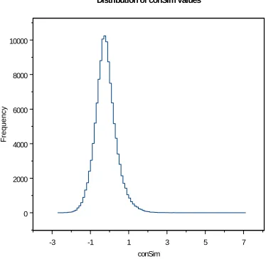
The first step is to compute the distribution of

1 2

( , )

conSim t t over a large random sample of

pairs of token types t1 and t2. For this purpose

sample of 302,515 pairs. This resulted in the value -1000, 180,845 times (60% of values). The remainder of the values, based on nonzero

1 2

( )

c

p t ∧t are distributed as shown in Figure 1.

Let τ denote the probability density for

1 2

( , )

conSim t t over random pairs t1 and t2 . Let

1 2

( , )

Sem t t denote the predicate that asserts that t1

and t2 are semantically related. Then our main

assumption which underlies the method is Postulate. For any nonnegative real number r

{

}

Q= conSim t t lexSim t t > ∧ ¬r Sem t t (7)

-3 -1 1 3 5 7

conSim 0

2000 4000 6000 8000 10000

Fr

e

que

nc

y

Distribution of conSim Values

Figure 1. Distribution of conSim values for the 40% of randomly selected token type pairs which gave values above -1000, i.e., for which

1 2

( ) 0

c

p t ∧t > .

has probability density function equal to τ .

This postulate says that if you have two token types that have some level of similarity as strings (lexSim t t( , )_{1 2} >r) but which are not semantically related, then lexSim t t( , )_{1 2} >r is just an accident and it provides no information about

1 2

( , )

conSim t t .

The next step is to consider a pair of real numbers

1 2

0≤ <r r and the set

{

}

1 2 1 2 1 1 2 2

( , ) ( , ) | ( , )

S r r = t t r ≤lexSim t t <r (8)

they define. We will refer to such a set as a lexSim

slice. According to our postulate the subset of

1 2

( , )

S r r which are pairs of tokens without a

se-mantic relationship will produce conSim values obeying the τ density. We compute the conSim

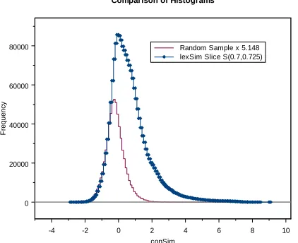
values and assume that all of those pairs that pro-duce a conSim value of -1000 represent pairs that are unrelated semantically. As an example, in one of our computations we computed a slice

(0.7,0.725)

S and found the lexSim value -1000 produced 931,042 times. In comparing this with the random sample which produced 180,845 values of -1000, we see that

931, 042 180,845=5.148 (9)

So we need to multiply the frequency distribution for the random sample (shown in Figure 1) by 5.148 to represent the part of the slice

(0.7,0.725)

S that represents pairs not semantically related. This situation is illustrated in Figure 2. Two observations are important here. First, the two curves match almost perfectly along their left edges for conSim values below zero. This suggests that sematically related pairs do not produce con-Sim scores below about -1 and adds some credibil-ity to our assumption that semantically related pairs do not produce conSim values of -1000. The second observation is that while the higher graph in Figure 2 represents all pairs in the lexSim slice and the lower graph all pairs that are not semanti-cally related, we do not know which pairs are not semantically related. We can only estimate the probability of any pair at a particular conSim score level being semantically related. If we let Ψ rep-resent the upper curve coming from the lexSim

slice and Φ the lower curve coming from the ran-dom sample, then (10) represents the probability

( ) ( ) ( )

( )

x x

p x

x

Ψ − Φ

=

Ψ (10)

that a token type pair with a conSim score of x is a semantically related pair. Curve fitting or regres-sion methods can be used to estimate p. Since it is reasonable to expect p to be a nondecreasing function of its argument, we use isotonic regres-sion to make our estimates. For a full analysis we set

0.5 0.025

i

and consider the set of lexSim slices

{

}

and determine the corresponding set of probability

functions

{ }

2.4 Learned Weights

Our initial step was to use the IDF weights defined in equation (6) and compute a database of all non-identical token type pairs among the 2,341,917 token types occurring in MEDLINE for which

1 2

( , ) 0.5

lexSim t t ≥ . We focus on the value 0.5

be-cause the similarity measure lexSim has the

-4 -2 0 2 4 6 8 10

conSim 0

20000 40000 60000 80000

F

re

que

nc

y

Random Sample x 5.148 lexSim Slice S(0.7,0.725) Comparison of Histograms

Figure 2. The distribution based on the random sample of pairs represents those pairs in the slice that are not semantically related, while the portion between the two curves represents the number of semantically related pairs.

property that if one of t₁ or t₂ is an initial seg-ment of the other (e.g., ‘glucuron’ is an initial segment of ‘glucuronidase’) then

1 2

( , ) 0.5

lexSim t t ≥ will be satisfied regardless of

the set of weights used. The resulting data in-cluded the lexSim and the conSim scores and consisted of 141,164,755 pairs. We performed a complete slice analysis of this data and based on the resulting probability estimates 20,681,478 pairs among the 141,164,755 total had a prob-ability of being semantically related which was greater than or equal to 0.7. While this seems like a very useful result, there is reason to be-lieve the IDF weights used to compute lexSim

are far from optimal. In an attempt to improve the weighting we divided the 141,164,755 pairs

into C₋₁ consisting of 68,912,915 pairs with a

conSim score of -1000 and C₁ consisting of the remaining 72,251,839 pairs. Letting wG denote the vector of weights we defined a cost function

(

)

(

)

1 2 1 1 2 1

1 2 ( , )

1 2 ( , )

( ) log ( , )

log 1 ( , )

t t C

t t C

w lexSim t t

lexSim t t −

∈

∈

Λ = −

+ − −

∑

∑

(12)

and carried out a minimization of Λ to obtain a set of learned weights which we will denote by

0

wG . The minimization was done using the L-BFGS algorithm (Nash and Nocedal, 1991). Since it is important to avoid negative weights we associate a potential v f( ) with each ngram feature f and set

( )

w f = v f . (13)

The optimization is carried out using the poten-tials.

The optimization can be understood as an at-tempt to make lexSim as close to zero as possible on the large set C₋₁ where conSim= −1000 and we have assumed there are no semantically re-lated pairs, while at the same time making lex-Sim large on the remainder. While this seems reasonable as a first step it is not conservative as many pairs in C1 will not be semantically

re-lated. Because of this we would expect that there are ngrams for which we have learned weights that are not really appropriate outside of the set of 141,164,755 pairs on which we trained. If there are such, presumably the most important cases would be those where we would score pairs with inappropriately high lexSim

scores. Our approach to correct for this possibil-ity is to add to the initial database of 141,164,755 pairs all additional pairs which pro-duced a lexSim t t( , )1 2 ≥0.5 based on the new

weight set w0

G

. This augmented the data to a new set of 223,051,360 pairs with conSim scores. We then applied our learning scheme based on minimization of the function Λ to learn a new set of weights w1

G

1 2

( , ) 0

conSim t t ≤ and C₁ those pairs with

1 2

( , ) 0

conSim t t > . We take this to be a

conserva-tive approach as one would expect semantically related pairs to have a similar context and satisfy

1 2

( , ) 0

conSim t t > and graphs such as Figure 2

support this. In any case we view this as a con-servative move and calculated to produce fewer false positives based on lexSim score recommen-dations of semantic relatedness. We actually go through repeated rounds of training and adding new pairs to the set of pairs. This process is con-vergent as we reach a point where the weights learned on the set of pairs does not result in the addition of a significant amount of new material. This happened with weight set wG₄ and a total accumulation of 440.4 million token type pairs.

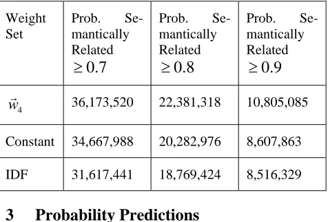
Table 1. Number of token pairs and the level of their predicted probability of semantic related-ness found with three different weight sets.

Weight Set

Prob. Se-mantically Related

0.7 ≥

Prob. Se-mantically Related

0.8 ≥

Prob. Se-mantically Related

0.9 ≥

4

wG 36,173,520 22,381,318 10,805,085

Constant 34,667,988 20,282,976 8,607,863

IDF 31,617,441 18,769,424 8,516,329

3 Probability Predictions

Based on the learned weight set w4

G

we per-formed a slice analysis of the 440 million token pairs on which the weights were learned and ob-tained a set of 36,173,520 token pairs with pre-dicted probabilities of being semantically related of 0.7 or greater. We performed the same slice analysis on this 440 million token pair set with the IDF weights and the set of constant weights all equal to 1. The results are given in Table 1. Here it is interesting to note that the constant weights perform substantially better than the IDF weights and come close to the performance of the w4

G

weights. While the w4

G

predicted about 1.5 million more relationships at the 0.7

prob-ability level, it is also interesting to note that the difference between the wG₄ and constant weights actually increases as one goes to higher probabil-ity levels so that the learned weights allow us to

Table 2. A table showing 30 out of a total of 379 tokens predicted to be semantically related to ‘lacz’ and the estimated probabilities. Ten en-tries are from the beginning of the list, ten from the middle, and ten from the end. Breaks where data was omitted are marked with asterisks.

Probability Semantic

Relation Token 1 Token 2

0.973028 lacz 'lacz

0.975617 lacz 010cblacz

0.963364 lacz 010cmvlacz

0.935771 lacz 07lacz

0.847727 lacz 110cmvlacz

0.851617 lacz 1716lacz

0.90737 lacz 1acz

0.9774 lacz 1hsplacz

0.762373 lacz 27lacz

0.974001 lacz 2hsplacz

*** *** ***

0.95951 lacz laczalone

0.95951 lacz laczalpha

0.989079 lacz laczam

0.920344 lacz laczam15

0.903068 lacz laczamber

0.911691 lacz laczatttn7

0.975162 lacz laczbg

0.953791 lacz laczbgi

0.995333 lacz laczbla

0.991714 lacz laczc141

*** *** ***

0.979416 lacz ul42lacz

0.846753 lacz veroicp6lacz

0.985656 lacz vglacz1

0.987626 lacz vm5lacz

0.856636 lacz vm5neolacz

0.985475 lacz vtkgpedeltab8rlacz

0.963028 lacz vttdeltab8rlacz

0.993296 lacz wlacz

0.990673 lacz xlacz

0.946067 lacz zflacz

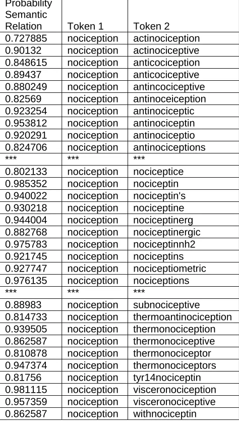
Table 3. A table showing 30 out of a total of 96 tokens predicted to be semantically related to ‘nociception’ and the estimated probabilities. Ten entries are from the beginning of the list, ten from the middle, and ten from the end. Breaks where data was omitted are marked with asterisks.

Probability Semantic

Relation Token 1 Token 2

0.727885 nociception actinociception

0.90132 nociception actinociceptive

0.848615 nociception anticociception

0.89437 nociception anticociceptive

0.880249 nociception antincociceptive

0.82569 nociception antinoceiception

0.923254 nociception antinociceptic

0.953812 nociception antinociceptin

0.920291 nociception antinociceptio

0.824706 nociception antinociceptions

*** *** ***

0.802133 nociception nociceptice

0.985352 nociception nociceptin

0.940022 nociception nociceptin's

0.930218 nociception nociceptine

0.944004 nociception nociceptinerg

0.882768 nociception nociceptinergic

0.975783 nociception nociceptinnh2

0.921745 nociception nociceptins

0.927747 nociception nociceptiometric

0.976135 nociception nociceptions

*** *** ***

0.88983 nociception subnociceptive

0.814733 nociception thermoantinociception

0.939505 nociception thermonociception

0.862587 nociception thermonociceptive

0.810878 nociception thermonociceptor

0.947374 nociception thermonociceptors

0.81756 nociception tyr14nociceptin

0.981115 nociception visceronociception

0.957359 nociception visceronociceptive

0.862587 nociception withnociceptin

A sample of the learned relationships based on the w4

G

weights is contained in

Table 2 and Table 3. The symbol ‘lacz’ stands for a well known and much studied gene in the E. coli bacterium. Due to its many uses it has given rise to myriad strings representing differ-ent aspects of molecules, systems, or method-ologies derived from or related to it. The results

are not typical of the inflectional or derivational methods generally found useful in studying the morphology of English. Some might represent misspellings, but this is not readily apparent by examining them. On the other hand ‘nocicep-tion’ is an English word found in a dictionary and meaning “a measurable physiological event of a type usually associated with pain and agony and suffering” (Wikepedia). The data in Table 3 shows that ‘nociception’ is related to the expected inflectional and derivational forms, forms with affixes unique to biology, readily apparent misspellings, and foreign analogs.

4 Discussion & Conclusions

There are several possible uses for the type of data produced by our analysis. Words semanti-cally related to a query term or terms typed by a search engine user can provide a useful query expansion in either an automatic mode or with the user selecting from a displayed list of options for query expansion. Many misspellings occur in the literature and are disambiguated in the token pairs produced by the analysis. They can be rec-ognized as closely related low frequency-high frequency pairs. They may allow better curation of the literature on the one hand or improved spelling correction of user queries on the other. In the area of more typical language analysis, a large repository of semantically related pairs can contribute to semantic tagging of text and ulti-mately to better performance on the semantic aspects of parsing. Also the material we have produced can serve as a rich source of morpho-logical information. For example, inflectional and derivational transformations applicable to the technical language of biology are well repre-sented in the data.

hu-man immunodeficiency virus. However, if ‘ive’ is also a feature of the token we may well be dealing with the word ‘hive’ which has no rela-tion to a human immunodeficiency virus. Thus a more complicated model of the lexical similarity of strings could result in improved recognition of semantically related strings.

In future work we hope to investigate the applica-tion of the approach we have developed to multi-token terms. We also hope to investigate the possi-bility of more sensitive lexSim measures for im-proved performance.

Acknowledgment This research was supported by the Intramural Research Program of the National Center for Biotechnology Information, National Library of Medicine, NIH, Bethesda, MD, USA.

References

Adamson, G. W., and Boreham, J. 1974. The use of an association measure based on character structure to identify semantically related pairs of words and document titles. Information Storage and Retrieval, 10: 253-260.

Alberga, C. N. 1967. String similarity and misspellings. Communications of the ACM, 10: 302-313.

Damashek, M. 1995. Gauging similarity with n-grams: Language-independent categorization of text. Sci-ence, 267: 843-848.

Findler, N. V., and Leeuwen, J. v. 1979. A family of similarity measures between two strings. IEEE Transactions on Pattern Analysis and Machine Intel-ligence, PAMI-1: 116-119.

Freitag, D. 2005. Morphology Induction From Term Clusters, 9th Conference on Computational Natural Language Learning (CoNLL): Ann Arbor, Michigan, Association for Computational Linguistics.

Hall, P. A., and Dowling, G. R. 1980. Approximate string matching. Computing Surveys, 12: 381-402.

Jacquemin, C. 1997. Guessing morphology from terms and corpora, in Belkin, N. J., Narasimhalu, A. D., and Willett, P., editors, 20th Annual International ACM SIGIR Conference on Research and Develop-ment in Information Retrieval: Philadelphia, PA, ACM Press, p. 156-165.

Jurafsky, D., and Martin, J. H. 2000. Speech and Lan-guage Processing: Upper Saddle River, New Jersey, Prentice Hall.

Means, R. W., Nemat-Nasser, S. C., Fan, A. T., and Hecht-Nielsen, R. 2004. A Powerful and General

Approach to Context Exploitation in Natural Lan-guage Processing, HLT-NAACL 2004: Workshop on Computational Lexical Semantics Boston, Massachu-setts, USA, Association for Computational Linguis-tics.

Monson, C. 2004. A framework for unsupervised natu-ral language morphology induction, Proceedings of the ACL 2004 on Student research workshop: Barce-lona, Spain, Association for Computational Linguis-tics.

Nash, S. G., and Nocedal, J. 1991. A numerical study of hte limited memory BFGS method and hte truncated-Newton method for large scale optimization. SIAM Journal of Optimization, 1: 358-372.

Schone, P., and Jurafsky, D. 2000. Knowledge-free in-duction of morphology using latent semantic analy-sis, Proceedings of the 2nd workshop on Learning language in logic and the 4th conference on Compu-tational natural language learning - Volume 7: Lis-bon, Portugal, Association for Computational Lin-guistics.

Sparck Jones, K. 1972. A statistical interpretation of term specificity and its application in retrieval. The Journal of Documentation, 28: 11-21.

Wicentowski, R. 2004. Multilingual Noise-Robust Su-pervised Morphological Analysis using the Word-Frame Model, SIGPHON: Barcelona, Spain, Asso-ciation for Computational Linguistics.

Wilbur, W. J., and Kim, W. 2001. Flexible phrase based query handling algorithms, in Aversa, E., and Man-ley, C., editors, Proceedings of the ASIST 2001 An-nual Meeting: Washington, D.C., Information Today, Inc., p. 438-449.

Willett, P. 1979. Document retrieval experiments using indexing vocabularies of varying size. II. Hashing, truncation, digram and trigram encoding of index terms. Journal of Documentation, 35: 296-305.

Xu, J., and Croft, W. B. 1998. Corpus-based stemming using cooccurrence of word variants. ACM TOIS, 16: 61-81.

Yarowsky, D., and Wicentowski, R. 2000. Minimally supervised morphological analysis by multimodal alignment, Proceedings of the 38th Annual Meeting on Association for Computational Linguistics: Hong Kong, Association for Computational Linguistics.