signal representations in NMF-based word recognition
Okko Räsänen
Department of Signal Processing and
Acoustics, Helsinki University of
Technology, Espoo, Finland
[email protected]
Joris Driesen
Department of Electrical Engineering,
Katholieke Universiteit Leuven, Leuven,
Belgium
[email protected]
Abstract
Segmental and fixed-frame signal representations were compared in different noise conditions in a weakly supervised word recognition task using a non-negative matrix factorization (NMF) framework. The experiments show that fixed-frame windowing results in better recognition rates with clean signals. When noise is introduced to the system, robustness of segmental signal representations becomes useful, decreasing the overall word error rate. It is shown that a combination of fixed-frame and segmental representations yields the best recognition rates in different noise conditions. An entropy based method for dynamically adjusting the weight between representations is also introduced, leading to near-optimal weighting and therefore enhanced recognition rates in varying SNR conditions.
1 Introduction
Structural characteristics of signal representations are an important aspect in all pattern discovery and speech recognition tasks. There are numerous different methods for describing speech signals that use different types of signal transformations, including, e.g., FFT, cepstra and LP-coefficients. These approaches describe local spectral properties of the signal as feature frames at a specific point in time. However, it is well known that also the way that temporal aspects of the signal are included in the analysis is important. Most approaches in speech recognition, including state-of-the-art HMMs, use fixed-frame windowing where the chosen features are extracted from approximately 20-25 ms long windows at fixed temporal intervals, e.g., every 10 milliseconds (see Gales
and Young, 2008).
Speech signals, however, have a very special temporal structure, which can be described in terms of hierarchically organized linguistically motivated units like utterances, words, syllables and phones. This structure has to exist in the speech signal in order for the receiver to be able to decode it. For example, human listeners are able to locate and segment phone-like segments in speech signal, although the reliability and accuracy of the location of phone-phone boundaries is often quite inaccurate (+/- 20 ms at best). Phone structure, or at least phone-like units, can then also be detected automatically using automatic segmentation algorithms that often use information about spectral changes in the signal in order to provide hypotheses about possible phone-boundary locations. These phone-like segments can then be described with chosen features to next levels of processing instead of fixed windowing, or the phone boundary information can be utilized in processing of fixed frame representations as was done in this study to form segmental representations. The way that temporal information is embedded in the feature stream has important implications for the next steps in the processing of the signals.
1.1 Properties of signal representations
In theory, the use of temporal segmental information should have several advantages. It synchronizes the feature stream to phonetically meaningful units in speech and the features can be extracted from desired temporal locations aligned with each segment. Phonetic synchrony facilitates the co-occurrence of subsequent phonetic units in temporally coherent manner (or at fixed lags in NMF) as the temporal deviations resulting from, e.g., different speaking rates or badly aligned windows are removed. This may aid pattern discovery methods, including NMF, in detection of recurring patterns (see Stouten et al., 2008). Segmental knowledge can be also used for compression of the feature data describing the signal, since each segment can be represented with a fixed number of features that incorporate all essential aspects of a segment. Segmental descriptions have the potential of being more robust in noisy situations when compared to fixed-frame representations, as they can integrate spectral information over large temporal units.
The use of fixed frame representations, on the other hand, has several advantages, too. It provides a stable stream of information about the speech signal without being affected by the underlying signal content. For example, in situations where a segmentation algorithm misses transitions from phone to another and therefore leads to deletions in the label sequence, the fixed frame representation provides systematical information of the spectral content in the transient signal. Temporal resolution of fixed frames is also good if the window step size is sufficiently small, which means that the quantized label sequences can describe short-term details in the signal whereas segmental information is often an ‘average’ description of the content of a detected phone-like unit.
2 Algorithms used in experiments
2.1 Signal representations
For the experiments, fixed-frame signal representations were first created using vector quantization (VQ) and then segmental information was utilized to derive segmental version of the representations. The signals were first pre-emphasized and then MFCC-features were extracted every 10 ms. Quantization of the signal
frames was performed using codebooks created by
k-means algorithm: one codebook for static MFCCs, one for Δ-, and one for ΔΔ- coefficients.
Corresponding VQ codebook sizes were 150, 150 and 100 labels, respectively. Each codebook was used as a separate input stream to the system.
Segmental information was provided using a blind segmentation algorithm that tracks sudden changes in the spectral content of the signal using cross-correlation of spectral frames. The algorithm detects approximately 75 % of the segmental boundaries defined in a manually annotated reference of a test-set in the TIMIT corpus (with maximum deviation of ± 20 ms; Räsänen, 2007). Segmental representations were created using the information about segmental boundaries to group fixed-frame representation into segments, and then compressing these groups of VQ labels in each stream into overall descriptions of the segments. In order to do this, a number of labels had to be chosen to represent each segment according to some decision criteria. Preliminary experiments indicated that the best method for picking up N
labels for each segment was to take the mode of labels (the most frequent label) inside each of the N pre-defined sub-segment. This smoothens out small variability inside segments and picks only the most dominant label for the chosen sub-segment. When one label was chosen to represent a segment, the mode was taken from labels between 5 % and 95 % of the entire segment duration. In case of two labels per segment, the segment was divided to two sub-segments from 5 % to 45 % and from 55 % to 95 % of segment duration and modes were taken from these sub-segments. In case of three labels, corresponding sub-segment ranges were from 5 % to 40 %, from 30 % to 70 %, and from 60 % to 95 % in terms of segment duration.
2.2 Word-learning algorithm
The idea of the method is as follows. Firstly, speech utterances are converted to a vectorized form by accumulating the co-occurrences of labels from a single stream (statics, velocity and acceleration) in the signal at different time offsets (lags) and putting them in a histogram. The histograms determined on the different label streams can be concatenated into a single high-dimensional vector. This representation, which is called the Histogram of Acoustic Co-occurrences (Van hamme 2008a), is very convenient for performing NMF, due to the non-negativeness of its elements and the fact that it is by approximation entirely composed of non-negative subparts, namely the HAC-representations of the words constituting the original utterances. Concretely, the NMF algorithm can be written as:
V ≈ W H (1)
in which V is a matrix, each column of which is the HAC-representation of an utterance from the input data. The columns of W contain non-negative parts that make up the data, and the columns of H contain the extent to which each of these parts is present in each utterance. If the inner dimension (i.e. the number of columns in W) of the factorization is cleverly chosen, typically a bit higher than the total number of different words to be learned in the data, the non-negative parts contained in the columns of W will approximately model the HAC-representations of those words after convergence (Van hamme, 2008a; Van hamme, 2008b).
Given an utterance from the test set, W can be used to calculate an activation level for each trained word. If our objective is to detect one single keyword in the utterances of the test set, the answer for each utterance will consist of the word that is maximally activated by this utterance.
3 Experiments
3.1 Material
A corpus recorded as a part of the ACORNS project1 was used. The chosen subset of the corpus (UK Y1) consists of 4000 English utterances spoken by four different native English speakers (two males). The sentences in the material simulate linguistic input to infants less than one year of age. Each utterance contains a keyword surrounded by
1 http://www.acorns-project.org
a carrier sentence (total 11 different keywords:
bath, book, bottle, car, daddy, mommy, nappy, shoe, telephone, Angus, Ewan). Each utterance is also paired with a meta-tag that indicates the presence of a keyword in the utterance. This simulates a multimodal information source in a situation where there is an object of interest in the environment and the learning agent is paying attention to it, making it possible to model acoustic content in association to some other information source. The training material consisted of 2999 randomly selected utterances and the test material of the remaining 1000 utterances (one signal was removed due to an apparent recording problem). In the evaluation, the algorithm had to provide most likely keyword for each utterance that was then compared to the manual annotation.
3.2 Baseline experiments
After training the system with the 2999 utterances in the training material using 10 ms fixed-frame VQ-labels, a baseline result of 0.1 % WER was obtained for word recognition. When information about segmental boundary locations was utilized, keyword recognition accuracy depended on the amount of labels used for describing each segment. WER of 3.2 % was obtained using 1 label per segment. Interestingly, with two labels, only WER of 3.3 % was obtained after profuse experimenting with parameters, whereas for three labels the WER decreased to 2.8 %, being slightly below one label condition.
speaking rate and long-range phonetic context. In case of three labels per segment, the segmental description contains both left and right context and a sort of “locus” description from the middle of each segment that seems to carry important information regarding the underlying phonetic content. This is still significantly worse than the 0.1 % WER baseline with fixed frame representation.
This concludes that the compression to segmental level descriptions loses some fine details in the speech signal that are meaningful in order to differentiate between words. Three labels per segment yields the best recognition results for segmental based signal representations but falls still far behind fixed frame accuracies.
However, using only one label per segment has a noteworthy impact on computational complexity of further processing, since the signal representation is compressed into approximately 1/11 (9.1 %) of the original 10 ms fixed-frame size. The accuracy with this approach is almost as good as with three labels per segment, but due to data reduction, it speeds up execution of the NMF algorithm greatly.
3.3 Introducing noise
In order to see how well the representations and NMF perform in noise, two different types of noise were introduced to the system: 1) white noise added to the acoustic input, and 2) artificial noise added to the already quantized label sequences. In these experiments, the fixed frame signal representations were compared with segmental labels with one label per segment (mode of fixed frame symbols inside the segment).
In the first noise condition, five levels of (white Gaussian) noise were added to the acoustic input before signal quantization. Corresponding signal-to-noise ratios were baseline level (set to 60 dB for visualization purposes), 40 dB, 30 dB, 20 dB, and 10 dB, mean noise level being computed over each utterance, including small silent portions in the beginning and in the end of the signals. For the remaining of this paper, this type of noise shall be called acoustic white noise (AWN).
The second type of noise, which shall be called
channel noise (CN), was introduced to the recognition process by directly scrambling the label sequences at random indices. A manually defined percentage of labels were changed to a
random label from the VQ codebook (using a uniform distribution). Five levels of SNR2 were used: ∞, 22dB, 8.5dB, 0dB, and -8.5dB (SNR =
10log([1-pscrambled]/pscrambled), where p
!
"
[0,1]). This type of scrambling simulates noise originating from somewhere inside the system, e.g., by errors in the transmission channel, and can be used to examine the nature of representations needed for reliable pattern discovery.It was also of interest whether fixed frame and segmental representations would contain complementary information. Therefore activations of keyword representations in NMF were
In addition, reliability of segmentation in noisy conditions is also a central issue in this type of comparison. Boundary detection accuracy of the used segmentation algorithm has been found reasonably robust at least down to 0 dB SNR, however leading to increase in over-segmentation rate as the noise becomes more dominating (still approximately 75 % of boundaries are correctly detected at SNR = 20 dB with less than 10 % of over-segmentation; Räsänen, in preparation). In order to confirm these findings in word recognition experiments instead of previous comparison to reference annotation, the segmentation was also performed in parallel with both noisy input and clean input to see differences between these two situations.
3.4 Experiments with acoustic white noise
The system, including VQ codebook and NMF representations, was first trained using clean speech and then tested in word recognition with VQ-labels produced at different levels of AWN. Figure 1 displays the results at different SNR levels. As can be seen, the results are very similar for both representations at SNR = 40 dB, but as the SNR goes further down, the segmental representation of the signal performs significantly better than the fixed 10 ms frames approach. Increasing and varying the lag parameter of NMF
2 Note that SNR is here defined as a ratio of corrupted
Figure 1: Word-error rates as a function of SNR for fixed frames labels every 10 ms, segmental labels (one label per phone-like segment) and these two combined in case of acoustic white noise. Combination of these representations has complementary value and increases the recognition accuracy.
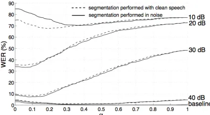
Figure 2: Word-error rates shown for different SNR
levels (acoustic white noise) as a function of representation weighting factor alpha. The left edge (alpha = 0) shows results for pure segmental representation whereas the right edge (alpha = 1) shows results using only fixed frame information.
did not affect the WER significantly from the original 50 ms and 90 ms lags in fixed-frame condition.
When word model activations from both representations are combined using eq. 2, WER further decreases, suggesting that they contain complementary information at all noise levels (alpha optimized separately for each SNR level). Figure 2 displays the word-error rates for combined representations at different SNR levels as a function of alpha, both with segmentation performed in noise (solid lines) and with clean speech (dashed lines).
As the fixed frame representation performs better at low noise levels, the optimal alpha for these levels is rather high. However, as soon as the SNR starts to drop, the optimal alpha starts to decrease fast. At very high noise levels the
Figure 3: Word-error rates in channel noise as a
function of SNR for fixed frames labels every 10 ms, segmental labels (one label per phone-like segment) and these two combined. Combination of these representations has complementary value and increases the recognition accuracy.
segmental descriptions seem to degrade badly and alpha shifts back towards fixed frames. This was found to be due to fact that at very high noise levels the vector quantization process tends to attract most of the feature vectors into a handful of
‘noise-like’ clusters. As these labels start to become the majority in the utterance related sequences, taking the mode of labels for all segments results in same (noise) symbols representing most of the segments. However, the overall recognition rates at 10 dB are extremely poor with all values of alpha.
Figure 2 also shows that the difference between blind segmentation performed in clean and noisy speech is not being significantly affected by the increase of noise all the way down to SNR = 20 dB. Only at SNR of 10 dB the degradation of segmentation quality becomes clearly visible in terms of recognition rate. This suggests that the information about segmental boundaries can be considered reliable at moderate white noise levels.
3.5 Experiments with channel noise
Figure 4: Word-error rates shown for different SNR levels (channel noise) as a function of alpha. The left edge (alpha α= 0) shows results for pure segmental
representation whereas the right edge (alpha = 1) shows results using only fixed frame information.
from the original 50 ms and 90 ms lags in fixed frame conditions or 1, 2, 3, 4, and 5 segments in segmental conditions. A value for alpha was again optimized for each SNR level separately by finding the value resulting in the minimum WER. Figure 4 shows the recognition rates at different noise levels and with different values of alpha.
A combination of the two different representations yields again the best recognition results, suggesting that the information about larger scale units (speech segments) can aid in the recognition process when the input is distorted. Next we will consider how this combination can be performed automatically when the signal conditions change.
4 Automatic weighting of
representations
4.1 Alpha in acoustic white noise
It was shown that combining fixed frame and segmental information is useful when noise is introduced to the system. But how does the system know how to weight small details (fixed frames) or larger units (segments), i.e., how can it automatically find a proper value for alpha in varying conditions when word-error rates are not available for optimization?
One method is to build a SNR dependent model for alpha so that value of alpha can be adjusted based on signal conditions. For on the fly estimation of SNR of the input, entropy is computed from the sequential label input X:
H(X)=" p(xi)lognp(xi)
i=1
n
#
(3)Figure 5: Entropy and optimal alpha values for acoustic
white noise are shown as a function of signal-to-noise ratio.
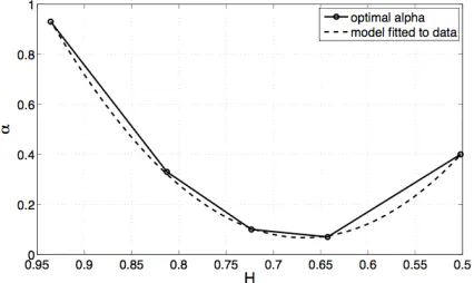
Figure 6: Optimal alpha values as a function of entropy
and the 2nd order polynomial fitted to data. A nearly optimal value for alpha in different noise conditions can be chosen dynamically by estimating entropy of the input sequences.
where n is the number of labels in the codebook and p is the probability distribution function of X that describes the frequency proportion of each symbol in the input. By measuring the entropy in different noise conditions, it is possible to find a mapping between SNR and the optimal alpha values. For white noise, entropy measured in the baseline SNR condition sets a maximum value for the entropy range, where H(X) = 1 would be obtained if signal content was entirely random (note that base of the logarithm is the size of the codebook). Figure 5 shows both entropy and the optimal alpha value as a function of SNR in the AWN condition. As the amount of noise increases, the entropy decreases as the noise-like clusters in the codebook start to become more probable.
By taking entropy estimates and optimal alpha values for the test signals at several noise levels, a good estimate for alpha can be described as a 2nd order polynomial function of entropy of the input sequences.
" =a2H2+a
The coefficients a2, a1, and a0 of the equation will depend on the used codebook, and therefore it is necessary to estimate entropy and WER values as a function of noise level and define these parameters in the development/training phase of the system. For VQ codebooks of size 150/150/100 (static, Δ,
and ΔΔ labels) used in the experiments, a2 = 12.07,
a1 = -16.1, and a0 = 5.4 were obtained. The parabolic fit to the data used in the experiments is extremely good (correlation > 0.999; figure 6) and therefore recognition rates are basically identical between entropy-based and manually optimized alpha, and are not therefore plotted separately (see fig. 3 for the results). In practice some deviation between these two may occur if the alpha is adjusted on the fly, depending on the temporal length of input used for estimating the entropy.
4.2 Alpha in channel noise
Entropy based alpha estimation can also be used in channel noise situation. In contrast to AWN, the entropy now increases as SNR decreases since labels at random locations become replaced with random labels. A reasonably good fit between entropy and alpha values can be obtained with a 1st order polynomial using eq. 4. However, even a more straightforward approach to select a proper alpha exists. It can be grossly approximated from figure 4 that the valleys of the curves are located in the middle section of the alpha range. Fixing α to
0.5 is then a trivial and computationally efficient method to combine information from both temporal resolutions in both clean sequences and noisy sequences.
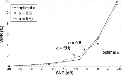
Figure 7: WER as a function of SNR for alpha
optimized for each noise level separately, calculated from signal entropy, and α = 0.5 for all noise levels. Weighting segmental and fixed frame information equally in all conditions leads to nearly same recognition accuracy as in optimized situation.
Figure 7 displays results from the recognition task in channel noise as was performed previously, now also including results with entropy based alpha estimation and the manually defined α. The
difference between recognition rates using optimal alpha values and alphas estimated from the input entropy are small. However, having fixed alpha of 0.5, that is, weighting the segmental and fixed frame information equally, leads to even better accuracy than the entropy based estimation. This suggests that this type of noise that does not take into account the spectral content of the speech, but uniformly affects entire quantized sequences, can be compensated by equally weighting fixed frame and segmental sized representations with NMF.
4.3 Discussion about noise experiments
An important finding here is that the information from larger temporal scales seems to become more and more important as the signal-to-noise ratio becomes worse (figures 2,4,5). Changes in the SNR of the input can be approximated with entropy after it is known how the entropy behaves at different levels of noise. This information can be then used to adjust the weight between scales dynamically.
When noise is introduced to the acoustic signal before vector quantization (e.g., external noise source), the quality of quantized labels suffers greatly as the spectral structure of the input becomes dominated by the noise, biasing the NMF word activations towards specific word models. It seems that integrating temporal information over phone-like speech segments helps to form more systematic representations than treating each small time-scale unit as a meaningful event in the presence of external (white) noise. Combining these two representation leads to better recognition accuracy than using either of them alone.
(more detailed) patterns match well with the small-scale representations, they dominate large-small-scale information in activation levels due to richness of information. When the small-scale patterns are distorted, previously learned large-scale patterns in the memory start to become more dominant. This linear weighting of cues has an interesting relation to perceptual processing in humans, where such summation of different cues embedded in the input takes place in, e.g., vision (Bruce et al., 2003; Oruc et al., 2003).
5 Conclusions
The use of segmental representations instead of fixed 10 ms frames degrades the recognition accuracy noticeably with clean speech. The magnitude of difference between these two is slightly surprising, as there are supposed to be several advantages of using segmental information, as was discussed in the introduction. However, it was found out that the segmental information is helpful in noisy conditions, adding robustness to the recognition decisions and therefore reducing the word-error rates. The weighting between segmental and fixed frame information can be estimated by utilizing entropy measure to the vector quantized labels. Parameters for this adaptive process have to be estimated in advance with well-defined input so that approximate entropy values for clean speech and several noise levels can be obtained.
In case of uniformly distributed random channel noise, simply using constant equal weight for both small and large temporal scales results in nearly optimal results. This may be because the strength of activation of internal representations in NMF at different temporal scales seems to follow the amount of previously learned structure available at these scales. This has striking similarity to theories of linear summation of cues from different scales of processing. Why this type of self-adjustment does not occur in case of AWN is not certain, but it may be due to the fact that the noise in quantization input changes the process systematically (reducing entropy). As such, it biases activations of internal representations towards a specific set of words instead of uniformly impeding all internal representations.
Acknowledgements
This research is funded as part of the EU FP6 FET project Acquisition of Communication and Recognition Skills (ACORNS), contract no. FP6-034362.
References
Vicki Bruce, Patrick R. Green and Mark A. Georgeson. 2003. Visual perception: Physiology, psychology and ecology. Lawrence Erlbaum Associates, UK. Louis ten Bosch, Hugo Van hamme and Lou Boves.
2008. A Computational Model of Language Acquistition: Focus on Word Discovery. In Proc. Interspeech, Brisbane, Australia.
Mark Gales and Steve Young. 2008. The Application of Hidden Markov Models in Speech Recognition. Foundations and Trends in Signal Processing. 1(3):195-304.
Daniel D. Lee and Sebastian H. Seung. 2001.
Algorithms for Non-Negative Matrix Factorization. In Advances in Neural Information Processing Systems ,13(1):556-562.
Ipek Oruç, Laurence T. Maloney and Michael S. Landy. 2003. Weighted linear cue combination with possibly correlated error. Vision Research, 43(23):2451-2468.
Okko J. Räsänen. 2007. Speech Segmentation and Clustering Methods for a New Speech Recognition Architecture. Master’s Thesis, TKK, Finland, http://lib.tkk.fi/Dipl/2007/urn010123.pdf. Okko J. Räsänen, Unto Laine and Toomas Altosaar, in
preparation. A Blind Speech Segmentation Algorithm Utilizing Non-linear Filtering and Temporal Masking of Spectral Frame Distances.
Veronique Stouten, Kris Demuynck and Hugo Van hamme. 2008. Discovering Phone Patterns in Spoken Utterances by Non-negative Matrix Factorization. IEEE Signal Processing Letters, 15(1):131-134.
Hugo Van hamme. 2008. HAC-models: a Novel Approach to Continuous Speech Recognition. In Proc. Interspeech, Brisbane, Australia.