Article
Modelling Distributed Systems in Distributed
Autonomous and Asynchronous Automata (DA
3
)
Wiktor B. Daszczuk 1,*
1 Institute of Computer Science, Warsaw University of Technology, Nowowiejska Str. 15/19, 00-665 Warsaw, Poland; [email protected]
* Correspondence: [email protected]; Tel.: +48-22-234-7812
Abstract: Integrated Model of Distributed Systems is used for modeling and verification. In formalism, the distributed system is modeled as a collection of server states and agent messages. The evolution of the system takes the form of actions that transform the global system configuration (states and messages) into a new configuration. Formalism is used in the Dedan verification environment for finding different kinds of deadlocks: communication deadlocks in the server view and resource deadlocks in the agent view. For other purposes, a conversion has been developed to equivalent models: to Petri nets for structural analysis and do Distributed Autonomous and
Asynchronous Automata (DA3) for easy graphical modeling in terms of system components. In
addition, it is possible to simulate a verified system on distributed components in DA3. The
automata have two forms: Server-DA3 (S-DA3) for the server view and Agent-DA3 (A-DA3) for the
agent view. DA3 formalism is compared to other concepts of distributed automata known from the
literature.
Keywords: distributed systems; distributed system modeling; distributed automata; graphical modeling; formal methods
1. Introduction
IMDS (Integrated Model of Distributed Systems [1]) is a formalism used to identify and verify distributed systems, in particular to detect deadlocks and check distributed termination. The system is built on servers - cooperating distributed nodes - and the cooperation takes the form of agents who perform distributed computing through migration between servers. The main element of IMDS is an action that has the server’s state and the agent’s message on the input and a similar pair on the output. The modelled distributed system can be decomposed into server processes consisting of sequences of actions threaded by server states. Alternatively, the same specification can be spread across agent processes that travel between servers. Agent processes are sequences of actions threaded by means of messages. Server processes communicate using messages while agent processes communicate using server states. Therefore, two decompositions correspond to communication duality. The IMDS formalism has been used, along with the model checking technique [2], to develop the Dedan program that finds various types of deadlocks in the verified system: communication deadlock (in the server view), resource deadlock (in the agent view), partial deadlock (in which a subset of system processes participate) and total deadlock (when all processes are involved). Similarly, the termination can be partial or total. Although Dedan’s main goal is deadlock and termination verification, the user may be interested in other properties of the distributed system, for example:
automatic conversion between the server view and the agent view,
observation of global transition graph,
structural properties of the system: structural conflicts, dead code, whether the system is
purely cyclic or not, etc.,
temporal properties other than deadlock: if the system is safe from some erroneous situation, if given situations are inevitable, etc.,
graphical definition of concurrent components of the system (servers or agents),
graphical simulation in terms of concurrent components rather than in terms of a global
graph.
In order to support these possibilities, additional facilities have been added to Dedan:
export of the model to the Petri net (ANDL format [3]), for static structural analysis [4]
under Charlie Petri net tool [5] ,
export to external model checkers for temporal analysis: Promela format (LTL model
checking in Spin [6]), SMV format (LTL and CTL model checking in NuSMV [7]), Timed Automata XML format (Timed CTL model checking in Uppaal [8]),
alternative formulation of a system as Distributed Automata (precisely – Distributed
Autonomous and Asynchronous Automata – DA3), to facilitate system specification and
simulation in terms of parallel components: automata represent server processes or agent processes.
This article focuses on a graphical automata-like model, equivalent to IMDS definition.
Servers in a distributed environment act asynchronously and make their decisions in autonomous manner. However, many modelling and verification formalisms use simultaneous activities of processes; like synchronous transitions on common symbols in Büchi automata [6] or Timed Automata [9], synchronization on send and receive operations in CSP [10], Occam [11] or Uppaal timed automata [8], synchronous operations on complementary input and output ports in CCS [10]. Several automata-based formalisms (including Büchi automata and Timed Automata) use synchronous coordination. There are several automata-based asynchronous models, they will be mentioned in Section 3. In IMDS, the autonomy of servers and agents is realized using asynchronous operations: sending the message to the server or setting the server’s state is the only way of influencing their behavior. The process autonomously decides if and when the communication would be accepted and what activities it would cause.
The contribution of this paper is the introduction of DAAA – Distributed, Asynchronous and
Autonomous Automata for modeling distributed systems (shortened to DA3 – D-triple-A or
DA-cubed). There are two versions of DA3, following the communication duality, Server DA3 (S-DA3) and
Agent DA3 (A-DA3). They are both equivalent to the IMDS specification and thus – to each other.
Automata are not the basic formalism of specification and verification, that is the role of IMDS. The automata are an interface to the graphical system specification as a set of cooperating state machines. At the same time, in the Dedan environment it is possible to simulate system operation in terms of automata and to follow the steps of the counterexample obtained from model checking.
The definition of IMDS is given in Section 2. The distributed automata DA3 are defined in Section
3. Also, the differences between DA3 and other notions of Distributed Automata in the literature are
discussed. The examples of Dedan operation on DA3 are described in Section 4. The equivalence
between IMDS and both versions of DA3 is shown in Section 5. Conclusions and further work are
covered in Section 6. Appendices present a larger example and operation of Dedan program.
2. Integrated Model of Distributed Systems (IMDS)
IMDS is defined in [1]. Here we use simplified version of IMDS, without dynamic process creation, which is suitable for conversion to finite automata, and for static model checking.
(MP) (MP) (2.1)
The set P is split into disjoint subsets attributed to servers in set S={s1,s2,...,sn}, while the set M is
split into disjoint subsets attributed to agents in set A={a1,a2,...,ak}. In an action λ∈Λ, λ=((m,p),(m’,p’)),
input and output state belong to the same server m,m’∈Mi, while input and output message belong
to the same agent p,p’∈Pj. A message is sent to a specific server to invoke its service, which is modelled
by a function target : M→S. In every pair (m,p) which is the input of an action λ, the server component must match: target(m)= si, p∈Pj, i = j.
Agents may be infinite or they may terminate in special actions of the form λ=((m,p),(p’)), where
an output message is absent.
The behavior of a distributed system is determined by its Labelled Transition System – LTS [12].
A node in LTS (we do not use a name ’state’ to avoid ambiguousness) is a configuration T of IMDS
model: set of current states of all servers and current messages of all agents (except for terminated ones). An initial configuration T0 contains initial states P0 and initial messages M0. An input configuration Tinp(λ) of an action λ =((m,p),(m’,p’)) contains m and p of its input pair (m,p) and the
output configuration Tout(λ) contains m’ and p’ of its output pair (m’,p’).
LTS = Q,q0,W where: (2.2)
Q = {T0,T1,...} (nodes)
q0 = T0 (initial node)
W = { (T, λ, T’) | λΛ, T=Tinp(λ), T’=Tout(λ) } (transitions)
Actions are executed in interleaving way (one action at a time [13]). Note that every server
performs its action autonomously (only the server’s state and the messages pending on this server are
considered). Also, the communication is asynchronous: a server process sends a message to some other server process (or an agent sets the server’s state for some other agent) regardless of the current situation of a process with which it communicates (and every other process). As a result, we may call the process autonomous and asynchronous.
The processes in the system are defined as sequences of actions. If two consecutive actions in a process are connected by a server state – it is a server process communicating with other server processes by means of messages (states are the carriers of server processes). If two consecutive actions in a process are connected by a message of an agent – it is an agent process communicating with other agent processes by means of servers’ states (agent messages are the carriers of agent processes).
Bi ={ λ∈Λ | λ =((m,p),(m’,p’)) ∨ λ =((m,p),(p’)), p,p’∈Pi } (2.3) Cj ={ λ∈Λ | λ =((m,p),(m’,p’)) ∨ λ =((m,p),(p’)), m,m’ ∈Mj }
The decomposition of a system into server processes is called a server view, the other one is an agent view.
B={ Bi|i =1...n } (2.4)
C={ Cj|j =1...k }
The examples of distributed systems modeled in IMDS may be found in [14]. In [15] the verification of Karlsruhe Production Cell is covered, where servers implement the devices in the cell, and agents implement metal plates that are processed. In Automatic Vehicle Guidance System [16] – servers implement road segment controllers and agents implement the vehicles.
3. Simple example – buffer
specification and verification of distributed systems the Dedan program was developed. For an action λ = ((m,p),(m’,p’)) a more convenient notation is used, in which a server state p is denoted as a pair (s,v), where s is a server and v is a value of a state, s∈S, v∈V. A message m is denoted as a triple (a,s,r), where a is an agent and r is a server’s sservice invoked by the message (a server may offer a number of services, for example wait and signal on a semaphore), a∈A, s∈S, r∈R. An action
To present the two views of a distributed system, a simple example of a buffer with producer and consumer agents (each one originating from its own server) is included in the listings below. First the server view follows. The notation is intuitional: server types are defined (lines 2, 9, 16). Formal parameters specify agents and other servers used. Every server includes states (l.3, 10), services (l.4, 11) and actions (l.6-7, 13-14). Then, server and agent variables are declared (l.17,18). The variables can have the same names as the types, they are distinguished by context. If a variable has
the same identifier as its type, a declaration variable:type may be suppressed to a single
identifier, as in the example. At the end, servers (l.20-22) and agents (l.23,24) are initialized, and variable names are bound with formal parameters of servers.
1. system BUF_server_view;
2. server: buf (agents Aprod,Acons; servers Sprod,Scons), 3. services{put, get},
4. states {no_elem,elem}, 5. actions {
6. {Aprod.buf.put, buf.no_elem} -> {Aprod.Sprod.ok_put, buf.elem}, 7. {Acons.buf.get, buf.elem} -> {Acons.Scons.ok_get, buf.no_elem}, 8. }
9. server: Sprod (agents Aprod; servers buf), 10. services{doSth,ok_put}
11. states {neutral,prod} 12. actions {
13. {Aprod.Sprod.doSth, Sprod.neutral} -> {Aprod.buf.put, Sprod.prod} 14. {Aprod.Sprod.ok_put, Sprod.prod} -> {Aprod.Sprod.doSth, Sprod.neutral} 15. }
16. server: Scons (agents Acons; servers buf), // similar to Sprod 17. servers buf,Sprod,Scons;
18. agents Aprod,Acons; 19. init -> {
20. Sprod(Aprod,buf).neutral, 21. Scons(Acons,buf).neutral,
22. buf(Aprod,Acons,Sprod,Scons).no_elem, 23. Aprod.Sprod.doSth,
24. Acons.Scons.doSth, 25. }.
The system converted to the agent view (this is done automatically by the Dedan program) is as follows.
1. system BUF_agent_view;
2. server: buf, services{put, get} states{no_elem, elem};
3. server: Sprod, services{doSth, ok_put} states{neutral, prod}; 4. server: Scons, services{doSth, ok_get} states{neutral, cons}; 5. agent: Aprod (servers buf:buf,Sprod:Sprod),
6. actions {
7. {Aprod.buf.put, buf.no_elem} -> {Aprod.Sprod.ok_put, buf.elem}, 8. {Aprod.Sprod.doSth, Sprod.neutral} -> {Aprod.buf.put, Sprod.prod}, 9. {Aprod.Sprod.ok_put, Sprod.prod} -> {Aprod.Sprod.doSth, Sprod.neutral}, 10. };
11. agent: Acons (servers buf:buf,Scons:Scons),// similar to Aprod 12. agents Aprod:Aprod,Acons:Acons;
13. servers buf:buf,Sprod:Sprod,Scons:Scons; 14. init -> {
15. Aprod(buf,Sprod).Sprod.doSth, 16. Acons(buf,Scons).Scons.doSth,
17. buf.no_elem, Sprod.neutral, Scons.neutral, 18. }
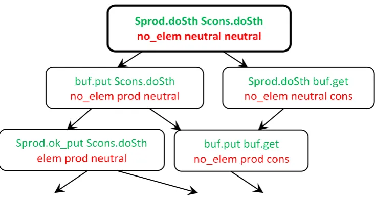
Figure 1. A fragment of LTS for the buffer system.
Of course, this LTS generated both from server view and from the agent view is identical, as they are projections onto servers and onto agents of a uniform system.
In Dedan program, communication and resource deadlocks may be identified and distributed termination may be checked. There is no deadlock in the example above, systems with deadlock are presented together with counterexamples in [14][15][16]. Also, a counterexample or other behaviour may be tracked in Deadn using a simulator. This simulation is performed over an LTS of a verified system. However, often a simulation should be performed over the components (servers and agents) of a verified system, shown separately and cooperating with each other. It is the reason of introducing Distributed Automata – an alternative formulation of IMDS system. Our distributed automata are equivalent to IMDS, but they allow for graphical definition and graphical simulation of distributed systems in terms of its components. Of course, the graphical form should preserve the autonomy of components and asynchrony of their behaviour. Also, communication dualism should be kept, therefore two forms of graphical specification are elaborated: one for the server view and the other for the agent view.
4.Distributed Autonomous and Asynchronous Automata (DA3)
In computer engineering practice,various forms of automata are used to express the behavior of concurrent components. There are two reasons: graphical representation and individual modeling of distinct components. UML state diagrams are the good example [17]. For a graphical representation of distributed systems, and for a simulation in terms of parallel components of a system, distributed
automata DA3 were invented. We claim that our distributed automata are better to describe
parallelism and cooperation in real distributed environment (with full asynchrony) than those enumerated below. Several different notions are called “distributed automata” in the literature.
1. Automata on distributed alphabets, communicating on common letters, based on
distributed [19]) are very close to Zielonka’s automata, they are simply equipped with time constraints and time invariants. Similar are CSP processes, synchronizing on ! and ? operations rather than on letters of input alphabet. The advantage of CSP lays in specifying the direction of communication (! is sending, ? is receiving), which should be supplied informally in the case Zielonka’s automata.
2. Close to Zielonka’s automata are Büchi automata. They differ in distinguishing some
states as accepting, used for LTL model checking (for instance in Spin [6]). They are called distributed automata in [24].
3. Message Passing Automata (MPA, called distributed automata in [25][26]) are really
distributed and asynchronous. They have ordered sets on letters waiting for acceptance, called buffers or queues.
4. Pushdown Distributed Automata (PDA) are equipped with local memories of input
symbols (stacks) [27].
5. The two former cases (MPA and PDA) are combined in [28][29] and called
distributed automata.
6. The automata that are synchronous in fact, with central synchronizing server. In such
an automaton, two independent actions are performed "simultaneously" by independent processors. The synchronizations between the processors are explicitly performed by a centralized processor: the synchronizer [30][31].
7. Grammar systems – languages for description of parallel systems, generated by
automata with certain interleaving rules. They are called distributed automata in [32].
8. Single large automaton split into distributed parts called distributed automata [33].
We introduce a new version of automata, equivalent to IMDS formalism. We call them Distributed
Autonomous, Asynchronous Automata - DA3 (D-triple-A or DA-cubed) to distinguish them from all
the listed formalisms, all called distributed automata. Our automata reflect the behavior of distributed components. The servers make decisions (perform actions) individually without any knowledge of other servers (autonomy) and messages are sent regardless of the states of target
servers (asynchrony). As there are two views of a distributed system in IMDS, two forms of DA3 were
developed – Server-DA3 and Agent-DA3 (S-DA3 and A-DA3).
4.1. Server automata S-DA3
An IMDS system in the server view may be shown as a set of communicating automata S-DA3
(Distributed Server Automata), similar to MPA (point 3 in the enumeration above):
States of a server are nodes (we use node instead of state to avoid ambiguity) of corresponding automaton.
An initial state of the server is an initial node of the automaton. Actions of the server process are transitions of the automaton. The automaton is Mealy-style [34], labels of the transitions in the
automaton have the form extracted from actions; an IMDS action λ=((m,p),(m’,p’)) is converted to a
transition from p to p’ with a label m/m’ (m is an input symbol conditioning the transition while m’ is
an output symbol produced on the transition); the transitions in the automaton of the server si are the
relation in PiM M Pi; of course m fulfil target(m)=si; note that "traditional" distinction between transition relation Pi M Pi and output function (Pi M Pi)→M is not held, because in the set of actions can contain nondeterministic actions λ1=((m,p),(m1,p’)), λ2=((m,p),(m2,p’)), m2m1. The
automaton is equipped with an input set – a set of input symbols pending, corresponding to a set of
pending messages at the server. Firing a transition (p,m/m’,p’) in the automaton of server s retrieves
the symbol m from the input set of this automaton and inserts the symbol m’ to the input set of an
automaton of the server s’ appointed by m’. An initial input set consists of initial messages of agents
directed to this server. The special agent-terminating action λ=((m,p),(p’)) is converted to a transition that does not produce any output symbol.
Formally, having the definition of S,A,V,R,P,M from IMDS (respectively: servers, agents, values,
Ƨ={ ƨi | i = 1...n }, where n is the number of servers in the set S. In the definition, exp(arg) is used for
powerset 2arg. An ith distributed server automaton is ƨi=(si,Pi,p0i,Fi,Xi,X0i), where:
si∈S – ith server,
Pi – set of nodes, states of si,
p0i∈Pi – initial node,
Fi={ (p1,m/m’,p2) for λ=((m,p1),(m’,p2)) or (p1,m/,p2) for λ=((m,p1),(p2)) | p1,p2∈Pi, aj ∈Am,m’∈Mj } – set of transitions (for ordinary action and agent-terminating action,
respectively),
Xi∈exp({m|target(m)=si}) – input set; Xi is a variable having a value of a set: a sender of a message (a transition delivering the message) inserts an element, execution of a transition removes an element, accordingly to rules for semantics below,
X0i∈exp({m|target(m)=si, m∈M0}) – initial input set.
The following conditions must hold, yet they are achieved by construction using the rules for semantics below:
m1∈Xi,m2∈Xj,m1∈Mk,m2∈Ml m1m2 kl: for any agent at most one message may exists in the
global configuration,
(p1,m/m’,p2)∈FiFjm’∈Fj: any output symbol is an input symbol of an automaton belonging
to Ƨ.
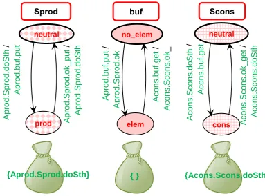
The automata are simpler on intuitive level, illustrated in Fig. 2 for the server automata of buffer
system. The input sets of the automata Xbuf, XSprod and XScons are shown at the bottom of the picture,
they change while the automata run.
no_elem
elem
A
co
n
s.
b
u
f.g
e
t
/
A
co
n
s.
S
co
n
s
.o
k
_
g
et
A
p
rod
.b
u
f.
p
u
t
/
A
p
rod
.S
p
rod
.o
k
_
neutral
prod
A
p
rod
.S
p
rod
.o
k_
p
u
t
/
A
p
rod
.S
p
rod
.d
o
S
th
A
p
rod
.S
p
rod
.d
o
S
th
/
A
p
rod
.b
u
f.
p
u
t
neutral
cons
A
co
n
s.
S
co
n
s
.o
k_
g
e
t
/
A
co
n
s.
S
co
n
s
.d
o
S
th
A
co
n
s.
S
co
n
s
.d
o
S
th
/
A
co
n
s.
b
u
f.g
e
t
{Aprod.Sprod.doSth}
{ }
{Acons.Scons.doSth}
Figure 2. Server automata for buffer system. Under the automata there are input sets with their initial values.
The semantics of Ƨ is defined as global node space ({ TƧ },TƧ 0,nextƧ), where { TƧ } is a set of global nodes, TƧ0 is an initial global node and nextƧ is a transition relation, defined as follows:
The global node of Ƨ is TƧ=((p1,X1),(p2,X2),...,(pn,Xn)) (current states and input sets of
If in TƧ there exists an ƨi in which (pi1,Xi), (pi1,m/m’,pi2)∈Fi, m∈Xi, target(m’)=sj then a
possible next global node T’Ƨ is:
𝑇Ƨ′=
((𝑝𝑘, 𝑋𝑘′)| {
𝑝′𝑘= 𝑝𝑘 𝑓𝑜𝑟 𝑘 ≠ 𝑖 𝑝′𝑘 = 𝑝𝑖2 𝑓𝑜𝑟 𝑘 = 𝑖
}
{
𝑋𝑘′ = 𝑋𝑘\{𝑚} ∪ {𝑚′} 𝑓𝑜𝑟 𝑖 = 𝑘 = 𝑗
𝑋𝑘′ = 𝑋𝑘\{𝑚} 𝑓𝑜𝑟 𝑘 = 𝑖 ≠ 𝑗 𝑋𝑘′ = 𝑋𝑘∪ {𝑚′} 𝑓𝑜𝑟 𝑘 = 𝑗 ≠ 𝑖 𝑋𝑘′ = 𝑋𝑘 𝑓𝑜𝑟 𝑖 ≠ 𝑘 ≠ 𝑗}
, 𝑘 =
1 … 𝑛) (4.1)
(the automaton ƨi changes its node to pi2, all other automata preserve their nodes; the
message m is extracted from the input set Xi of the automaton ƨi, the continuation
message m’ is inserted into the input set Xj of the automaton ƨj appointed by m’, all
other input sets remain unchanged; the special case is for (i = k = j, first case), where a server si sends a message to itself).
If in TƧ there exists an ƨi in which (p1,Xi), (pi1,m,pi2)∈Fi, m∈Xi (message m terminates the
agent) then a possible next global node is:
𝑇Ƨ′= ((𝑝𝑘, 𝑋𝑘′)| {
𝑝′𝑘= 𝑝𝑘 𝑓𝑜𝑟 𝑘 ≠ 𝑖 𝑝′𝑘 = 𝑝𝑖2 𝑓𝑜𝑟 𝑘 = 𝑖
} { 𝑋𝑘
′ = 𝑋
𝑘\{𝑚} 𝑓𝑜𝑟 𝑘 = 𝑖 𝑋𝑘′ = 𝑋𝑘 𝑓𝑜𝑟 𝑘 ≠ 𝑖
} , 𝑘 =
1 … 𝑛) (4.2)
(the automaton ƨi changes its node to pi2, all other automata preserve their nodes; the
message m is extracted from the input set Xi of the automaton ƨi, all other input sets
remain unchanged).
The initial global node is TƧ0 =((p01,X01),(p02,X02),...,(p0n,X0n)).
For given global node TƧ, transition relation nextTƧ(TƧ) is a set of pairs (TƧ,T’Ƨ). The
transition relation nextƧ = ∪TƧnextTƧ(TƧ). If for TƧ there exist multiple possible next global
nodes, one of them is chosen in nondeterministic way.
A global graph of Ƨ cooperation may be elaborated in such a way that nodes are global nodes TƧ , and
edges are transitions in automata ƨi. Of course, this graph is analogous to the LTS of IMDS system:
global nodes contain states of all servers, input symbol (message) of a transition should be attributed to a source global node, while output symbol (message) to a target global node. The fragment of a global node space for the buffer system is presented in Fig. 3.
The initial sates of servers are in bold ovals. Server names are omitted in the state labels, because they are identical for all states in given server automaton. As the automata may be treated as patterns for creation of many instantiations of similar automata, agent and server formal parameters should be added for server types automata:
Sprod(Aprod,buf), buf(Aprod,Acons,Sprod,Scons), Scons(Acons,buf)
Every automaton is equipped with the input set of pending messages:
Xbuf ∈exp({(Aprod,buf,put),(Acons,buf,get)}).
XSprod ∈exp({(Aprod,Sprod,doSth),(Aprod,Sprod,ok_put)}). XScons∈exp({(Acons,Scons,doSth),(Acons,Scons,ok_get)}).
Note that both messages in the base set of XSprod cannot be included in XSprod at the same time, as they
belong to the same agent, likewise in the case of XScons. The initial input sets are:
X0buf = ∅,
X0Sprod = {(Aprod,Sprod,doSth)}, X0Scons = {(Acons,Scons,doSth)}.
The S-DA3 are similar to Message Passing Automata. The difference is in the ordering of messages on
the input of the automaton: in MPA pending messages are ordered in the input queue (or input
buffer) [25][26], while in S-DA3 any message form the input set may cause a transition (no ordering).
If the input buffers are bounded, a deadlock may occur because of all processes sending to full buffers. Such a situation occurs when the size of buffers is taken too small [35]. IMDS helps to overcome this problem by posing an accurate limit for the input set maximum size (or the input buffer in the implementation): it is simply the number of agents. More precisely, it is the number of agents having their messages in the base set of the input set of the automaton.
4.2. Agent automata A-DA3
An IMDS system in the agent view may be shown as a set of communicating automata A-DA3
(Agent Distributed Autonomous and Asynchronous Automata). We use term node in these automata instead of state, because states ate attributed to servers in IMDS and it may be misleading. The
A-DA3 automata are similar to Timed Automata with variables used in Uppaal [8] (but we consider
only timeless systems here):
Messages of an agent are nodes of a corresponding automaton.
An initial message of the agent is an initial node of the automaton.
Actions of the agent process are transitions of the automaton.
The automaton is Mealy-style [34]; the labels of the transitions in the automaton have the
form extracted from actions; an IMDS action λ=((m,p),(m’,p’)) is converted to a transition (m,p/p’,m’) from m to m’ with a label p/p’ (p is an input symbol conditioning the transition
while p’ is an output symbol produced on the transition; as before a transition relation in
MiP Mi and output function (MiP Mi)→P are replaced by a single relation in MiP P Mi due to possible nondeterminism in the set of actions: λ1=((m,p),(m’,p1)), λ2=((m,p),(m’,p2)), p2p1.
For an agent-terminating action λ=((m,p),(p’)), a special terminating node t in the automaton is added as transition destination node, and the transition is of the form (m,p/p’,t). For t no outgoing transition is defined.
The system is equipped with a global input vector – the vector of current input symbols
– server’s states. Firing a transition (m,p/p’,m’) in the automaton replaces the symbol p in
the vector with the symbol p’. The initial global input vector consists of initial states of
all automata.
Formally, having the definition of P,M,S,A,V,R from IMDS (respectively: states, messages, servers,
general quantifier) of k distributed agent automata Ʉ = { ɐi | i =1...k }, where k is the number of agents
in the set A, and n is the number of servers in the set S (used in the definition of the agent automaton below). An ith distributed agent automaton is ɐi = (ai,Mi,m0i,tɐi,Gi,Y,Y0), where:
ai – ith agent,
Mi
∪
{tɐi} – set of nodes, tɐi is the destination node if the agent ɐi terminates (it appears interminating transition),
m0i∈Mi – initial node,
Gi ={ (m1,p/p’,m2) for λ=((m1,p),(m2,p’)) or (m1,p/p’,tɐi) for λ=((m1,p),(p’)) | m1,m2∈Mi, sj∈Sp,p’∈Pj } – set of transitions,
Y =[p1,...,pn] | pj∈Pj – global input vector (common for all ai in the system); Y is a vector of
variables, Y/i is the ith position of Y, every variable Y/i has a range over a set of states of
server sj: an action changes value of the variable at the position of its server: accordingly to rules for semantics below; ,
Y0 = [p01,...,p0n] | pj∈Pj, pj∈P0 – initial global input vector, consisting of initial states of all
servers.
Sprod.
doSth
S
p
rod
.p
rod
/
S
p
rod
.n
e
u
tra
l
S
prod.ne
ut
ra
l
/
S
p
rod
.p
rod
Sprod.
ok_put
b
u
f.
n
o
_
e
le
m
/
b
u
f.
e
lem
Scons.
doSth
.co
n
s /
.n
e
u
tra
l
.ne
ut
ra
l
/
.
Scons.
ok_get
bu
f.
ele
m
/
b
u
f.
n
o
_
e
le
m
Sprod
buf
Scons
neutral
no_elem
neutral
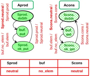
Figure 4. Agent automata for buffer system. Under the automata there is the global input vector
with its initial content.
The semantics of Ʉ is defined as global node space ({ TɄ },TɄ0,nextɄ), where { TɄ } is a set of global nodes, TɄ0 is initial global node and nextɄ is a transition relation, defined as follows:
The global node of Ʉ is TɄ={m1,...,mk,Y}, mi∈Mi ∪ {tɐi}. If in TɄ there exists mi, for which
there exists (mi,p/p’,mj)∈Gi, p,p’∈Px (message mi causes a change of a state from p to p’ in a
server sx, target(mi)=sx, and a message mj to a server sy, target(mj)=sy is issued) then a possible next global node is:
𝑇Ʉ′∶ ∀𝑚𝜖𝑇Ʉ { 𝑚 = 𝑚𝑖∧ 𝑚 = 𝑚𝑗 𝑚𝑖∈ 𝑇Ʉ′ 𝑚 = 𝑚𝑖∧ 𝑚 ≠ 𝑚𝑗 𝑚𝑗∈ 𝑇Ʉ′ 𝑚 ≠ 𝑚𝑖 𝑚𝑖∈ 𝑇Ʉ′ } ; 𝑌′= [𝑝
1, … , 𝑝𝑛] | 𝑝𝑘= {{
𝑌/𝑘 𝑓𝑜𝑟 𝑘 ≠ 𝑥
𝑝′ 𝑓𝑜𝑟 𝑘 = 𝑥 } , 𝑘 = 1 … 𝑛
(the automaton ɐi i changes its node to mj, all other automata preserve their nodes;
the state p in input vector Y is replaced by p’ in the position of the server sx, appointed
by p and p’, all other elements of the vector Y remain unchanged).
If in { TɄ } there exists mi, for which there exists (mi,p/p’,tɐi)∈Gi, p,p’∈Px (message mi is a
last message in the run of agent ai, then the agent terminates, a sever sx appointed by the
message mi, target(mi)= sx changes its state from p to p’) then a possible next global node
is:
𝑇
Ʉ′∶ ∀
𝑚𝜖𝑇Ʉ{
𝑚 = 𝑚
𝑖
𝑚
𝑖∉ 𝑇
Ʉ′
𝑚 ≠ 𝑚
𝑖
𝑚
𝑖∈ 𝑇
Ʉ′} ;
𝑌
′= [𝑝
1
, … , 𝑝
𝑛] | 𝑝
𝑘= {
𝑌/𝑘 𝑓𝑜𝑟 𝑘 ≠ 𝑥
𝑝
′𝑓𝑜𝑟 𝑘 = 𝑥
} , 𝑘 = 1 … 𝑛
(4.4)
(the automaton ɐi changes its node to tɐi all other automata preserve their nodes; the
state p in Y is replaced by p’ as above). The initial global node TɄ0 ={m01,...,m0n,Y0}. For
given global node TɄ, transition relation nextTɄ(TɄ) is a set of pairs (TɄ,T’Ʉ). The
transition relation nextɄ =
∪
TɄ nextTɄ(TɄ). In given global node TɄ, if there aremultiple next nodes possible, one of them is chosen in nondeterministic way.
Distributed agent automata for the buffer system are illustrated in Fig. 4. The initial messages of the agents are in bold ovals. Agent identifies are omitted in message labels (nodes of the automata), because they are identical for all messages in given agent type automaton. Below is the global input vector of current states of servers:
Y = [(Sprod,value∈{neutral,prod}), (buf,value∈{no_elem,elem}), (Scons,value∈ {neutral,cons})].
The initial content of the global input vector is:
Y0 =[(Sprod,neutral),(buf,no_elem),(Scons,neutral)].
A global graph of Ʉ cooperation may be elaborated analogously to the graph of Ƨ: nodes of the global
graph are global nodes TɄ , and edges are transitions in automata ɐi. This graph is analogous to the
global graph of S-DA3 and to the LTS of IMDS system (global nodes contain messages of all agents,
input symbol/state of a transition should be attributed to a source global node, while output symbol/state to a target global node).
5. Equivalence of the formalisms
In this section we show the equivalence of the IMDS model with both automata-based models: S-DA3
and A-DA3. the equivalence is based on similar LTS structures, i.e., every node of LTS – including
initial ones – should contain the same elements (states and messages) as corresponding nodes in other LTS’es. That is, corresponding nodes should contain exactly the same sets of elements, but in various
forms: set elements in IMDS, nodes and elements of input sets of S-DA3, nodes and elements of input
vector in A-DA3, except terminating nodes. Furthermore, the transitions should join corresponding
nodes in all LTS’es. To show the equivalence, the rule of obtaining Tout(λ) from Tinp(λ) for the action λ
is needed. This rule comes directly ftom the definition of IMDS:
λ=((m,p),(m’,p’)) Tinp(λ) {m,p} Tout(λ)=Tinp(λ)\{m,p} ∪ {m’,p’} (5.1) λ=((m,p),(p’)) Tinp(λ) {m,p} Tout(λ)=Tinp(λ)\{m,p} ∪ {p’}
1. LTS node
IMDS: T={ p,m | p∈P, m∈M }, Every p from a different s every m from a different a except terminated a,
S-DA3: TƧ=((p1,X1),...,(pn,Xn)) Every p from a different s – from definition in TƧevery s
the same a (will be shown later). No X can contain m appointing a terminated a (will be shown later),
A-DA3: TɄ={m,m’,m’’,...,Y} Every m appoints different a – from definition in TɄ every a
participates, except terminated ones (will be shown later). For every pair m1,m2 both
cannot appoint the same a (will be shown later). No m can appoint a terminated a (will
be shown later). Y contains the states of all servers – from definition.
2. Initial LTS node
IMDS: T0={ p0,m0 | p0∈Pini, m0∈Mini },
S-DA3: TƧ0 =((p01,X01),...,(p0n,X0n)) Every p from a different s – from definition. Every s
participates – from definition. For every pair X01,X02 both cannot contain m appointing
the same a (from definition, as X0i contains m0 for a starting from the server si, and ai∈Acard(Mi ∩ Mini)=1 (the initial set of messages contains exactly one message for every
agent). Every a has its m0 in some X0i – this from which the agents starts (X0i are indexed by servers and every m0 belongs to some Mi).
A-DA3: TɄ = {m01,...,m0k,Y0} In every pair m1,m2 both cannot appoint the same a (from
definition, as ai∈Acard(Mi ∩ Mini)=1 (the initial set of messages contains exactly one
message for every agent). No m can be tɐ – from definition. Every element of Y0 appoints
different server – from definition.
3. Transition in LTS (regular)
IMDS: (Tinp(λ),λ,Tout(λ)) | λ∈Λ, λ=((m,p),(m’,p’))
S-DA3: From TƧ there exists a regular transition (p,m/m’,p’) to T’Ƨ corresponding to λ=((m,p),(m’,p’)), in the automaton ƨi of the server si appointed by p to the state p’,
retrieving the message m from Xi and inserting a message m’ to Xj appointed by m’.
Both messages m,m’ belong to the agent a. If TƧ corresponds to Tinp(λ), then according to
(4.1) in T’Ƨp is replaced by p’ and in the union of all Xim is replaced by m’, and all other
states and messages are equal in TƧ and T’Ƨ, which fulfils the rule of obtaining Tout(λ) from Tinp(λ).
For every regular λ =((m,p),(m’,p’)) having p on input such a transition (p,m/m’,p’) exists in automaton ƨi appointed by p, and no other than for such λ transition exists, so it exactly
corresponds to the set of regular actions having p on input.
In every regular transition in ƨi, the set of servers is preserved (as p and p’ appoint the
same server) and the set of agents (as m and m’ appoint the same agent).
A-DA3: From TɄ there exists a regular transition (m,p/p’,m’) to T’Ʉ corresponding to λ=(m,p),(m’,p’)), in the automaton ɐi of the agent ai appointed by m to the message m’,
replacing the state p in Y by the state p’ of the same server s appointed by states p,p’ (in the position of the server s in Y).
If TɄ corresponds to Tinp(λ), then according to (4.3) in T’Ʉm is replaced by m’ and p in Y
is replaced by p’, and all other states and messages are equal in TɄ and T’Ʉ, which fulfils
the rule of obtaining Tout(λ) from Tinp(λ).
For every regular λ =((m,p),(m’,p’)) having m on input such a transition (m,p/p’,m’) exists in automaton ɐi appointed by m, and no other than for such λ transition exists, so it
exactly corresponds the set of regular actions having m on input.
In every regular transition in ɐi, the set of agents is preserved (as m and m’ appoint the
same agent) and the set of servers (as p and p’ appoint the same server).
4. Transition in LTS (agent-terminating)
IMDS: (Tinp(λ),λ,Tout(λ)) | λ∈Λ, λ=((m,p),(p’))
S-DA3: From TƧ there exists a terminating transition (p,m/,p’) to T’Ƨ corresponding to λ=((m,p),(p’)), in the automaton ƨi of the server si appointed by p, to the state p’, retrieving
the message m from Xi. The message m belongs to an agent a.
If TƧcorresponds to Tinp(λ), then according to (4.2) in T’Ƨp is replaced by p’ and m is
of obtaining Tout(λ) from Tinp(λ) (terminating action).
For every terminating λ =((m,p),(p’)) having p on input such a transition (p,m/,p’) exists in automaton si appointed by p, and no other than for such λ transition exists, so it exactly
corresponds the set of terminating actions having p on input.
In every terminating transition in si, the set of servers is preserved (as p and p’ appoint
the same server) and the set of agents in T’Ƨ is smaller by the agent appointed by m.
Consequently, there is no way to reestablish a terminated agent.
A-DA3: From TɄ there exists an agent a terminating transition (m,p/p’,tɐ) to T’Ʉ
corresponding to λ = ((m,p),(p’)), in the automaton ɐi of the agent ai appointed by m, to
the message m’, replacing the message m by tɐi.
The state p belongs to a server s. If TɄ corresponds to Tinp(λ), then according to (4.4) in T’Ʉ m is replaced by tɐi and p is replaced in Y by p’, all other states and messages are equal in TɄ and T’Ʉ, which fulfils the rule of obtaining Tout(λ) from Tinp(λ) (terminating action).
For every terminating λ =((m,p),(p’)) having m on input such a transition (m,p/p’,tɐ) exists
in automaton ɐi appointed by m, and no other than for such λ transition exists, so it
exactly corresponds the set of terminating actions having m on input.
In every terminating transition in ɐi, the set of servers is preserved (as p and p’ appoint
the same server) and the set of agents in T’Ʉ is smaller by the agent appointed by m, which
is replaced by tɐi. Consequently, there is no way to reestablish a terminated agent.
5. Semantics of LTS
IMDS: Interleaving, nondeterministic,
S-DA3: Interleaving, nondeterministic,
A-DA3: Interleaving, nondeterministic.
6. Conclusions and further work
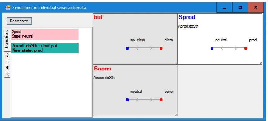
Figure 5. Simulation over SDA3 automata. Every automaton has its own sub-window, a chosen
automaton has blue caption and light background. On the left, current state of the chosen automaton and a list of possible transitions are displayed.
The Dedan program supports an engineer in specification of distributed systems and their verification for deadlocks freeness and distributed termination. If a deadlock occurs, a sequence diagram of messages and states is generated, leading from the initial configuration to the deadlock. If the deadlock is not total, the servers/agents taking part in the deadlock is are shown. Distributed automata (in S-DA3 or in A-DA3 version) allow to design the system in graphical form, and to
counterexample may be observed as a sequence of transitions in cooperating DA3 automata.
Engineers are familiar with the notion of automata (S-DA3 are similar to Message Passing Automata
[25][26] and A-DA3 are like Timed Automata with global variables of Uppaal [8]) and they may be
naturally used in distributed systems design. For example, some models of transport cases were modeled. Observation of the server view is equivalent to exchange of messages between road segment controllers that automatically lead the vehicles on the roads [16]. In the agent view, it is the observation of vehicles moving over the road, with interactions to other vehicles occupying some segments of the road. Possible deadlocks in communication may by easily identified, and the verifier shows the behavior of vehicles leading to a deadlock as transitions of DA3 automata. Table 1
compares the features of a distributed system, observed in equivalent formalisms: IMDS and DA3.
Table 1. Verification facilities in the three equivalent formalisms.
Formalism: IMDS S-DA3 A-DA3
Main features
Specification, model checking, simulation
Graphical input, simulation
Graphical input, simulation
Notions state node element of global input
vector, input/output symbol on transitions
message element of input set,
input/output symbol on transitions
node
configuration global node global node
action transition transition
initial state initial node initial element of global
input vector
initial message initial element of input set initial node
initial configuration initial nodes and initial
input sets of all automata
initial nodes and initial global input vector Labeled Transition
System
Global node space: all states and input sets in global nodes, input and
output symbols on
transitions
Global node space: all messages and global input vector in global nodes, input and output symbols on transitions
Features Resource deadlock
Communication
deadlock
Partial deadlock
Total deadlock
Partial distributed
termination
Total distributed
termination
Counterexamples/
witnesses
Configuration space
inspection
Simulation over
configuration space
Graphical definition
of a system (as servers)
Simulation over
individual server automata
Counterexample
projected onto individual server automata
Counterexample–
guided simulation
Graphical definition
of a system (as agents)
Simulation over
individual agent automata
Counterexample
projected onto individual agent automata
Counterexample–
guided simulation
Timed DA3 automata, in which time constraints will be added to actions and message
passing. This will allow to check for deadlocks in real time-dependent systems.
Probabilistic DA3 automata allowing to identify a probability of a deadlock if the
alternative actions in system processes are equipped with probabilities.
Language-based input – elaboration of two languages for distributed systems
specification: one for the server view (exploiting locality in servers and message passing) and the other one for the agent view (exploiting travelling of agents and resource sharing in distributed environment); a preliminary version of a declarative language-based preprocessor for a server view of verified systems is developed by the students of ICS, WUT (Institute of Computer Science, Warsaw University of Technology).
Agent’s own actions – equipping the agents with their own sets of actions, carried in their
“backpacks”, parametrizing their behavior; this will allow for modelling of mobile agents (agents carrying their own actions model code mobility) and to avoid many server types in specification, differing slightly.
The Dedan environment is successfully used in operating systems laboratory in ICS, WUT. The students verify their solutions of synchronization problems. Graphical definition of component automata and simulation over distributed automata supports the procedure of verification.
Supplementary Materials: The Dedan program is available online at http://staff.ii.pw.edu.pl/dedan/files/DedAn.zip, examples at http://staff.ii.pw.edu.pl/dedan/files/examples.zip. Funding: This research received no external funding.
Conflicts of Interest: The author declares no conflict of interest.
Appendix A - Practical example of DA3: Automatic Vehicle Guidance System
Road Marker E1
Road Marker M
Road Marker E2 Warehouse Lot E2 Warehouse Lot E1
Warehouse Lot M
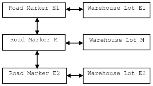
Figure A1. Structure of road segment controllers.
The buffer example is a tiny one, just to present the main ideas. Now we will introduce the Automatic Vehicle Guidance System (AVGS) from [16]. The system consists of road markers and warehouse lots, presented in Fig. A1, communicating with each other in order to guide autonomous moving
platforms (AMPs) from Lot_E1 to Lot_E2 or reverse way. There is an obvious conflict in MarkerM,
and it may be defeated using the LotM as a staggered arrangement. There are six servers representing
<i=1..N>AMP[i].lotE.start /
AMP[i].mE.tryL
<i=1..N>
AMP[i].lotE.try
/ AMP[i].mE.okL
<i=1..N>AMP[i].lotE.ok /
AMP[i].mE.takeL
<i=1..N>AMP[i].lotE.take /
!
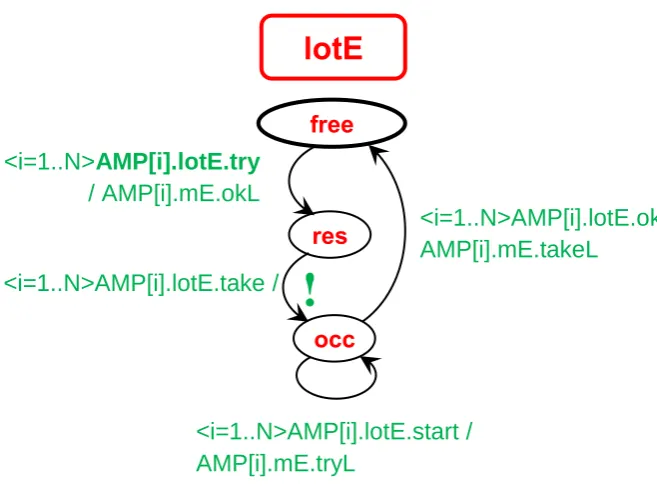
Figure A2. Server automaton of lotE server type.
The server view describes the system from the point of view of communicating controllers. The code of AVGS in IMDS source notation is given below.
1. #DEFINE N 2
2. server: mE (agents AMP[N]; servers mM,lotE), 3. //Edge Road Marker 4. ...
19. server: mM (agents AMP[N]; servers mE[2],lotM), 20. //Middle Road Marker
21. services {tryE[2],tryL[2],okE[2],notE[2],okL[2], takeE[2],takeL[2],switch[2]}, 23. states {free,resE[2],resL[2],occ},
24. actions {
25. //going to ME1 or ME2
26. <i=1..N><j=1..2> {AMP[i].mM.tryE[j], mM.free} -> {AMP[i].mE[j].okM[j], mM.resE[j]}, 27. <i=1..N><j=1..2> {AMP[i].mM.takeE[j], mM.resE[j]} -> {AMP[i].mM.switch[3-j], mM.occ}, 28. <i=1..N><j=1..2> {AMP[i].mM.switch[j], mM.occ} -> {AMP[i].mE[j].tryM[j], mM.occ}, 29. <i=1..N><j=1..2> {AMP[i].mM.okE[j], mM.occ} -> {AMP[i].mE[j].takeM, mM.free}, 30.
31. //on a way to ME1 or ME2 may go to LE if MEi occupied
32. <i=1..N><j=1..2> {AMP[i].mM.notE[j], mM.occ} -> {AMP[i].lotM.try[j], mM.occ}, 33. <i=1..N><j=1..2> {AMP[i].marker2.okL[j], mM.occ} -> {AMP[i].lotM.take[j], mM.free}, 34.
35. //going from PL2 - goes to RM1(mE[1]) or RM3(mE[2])
36. <i=1..N><j=1..2> {AMP[i].mM.tryL[j], mM.free} -> {AMP[i].lotM.ok[j], mM.resL[j]}, 37. <i=1..N><j=1..2> {AMP[i].mM.takeL[j], mM.resL[j]} -> {AMP[i].mE[j].tryM[j], mM.occ}, 38. <i=1..N><j=1..2> {AMP[i].mM.okE[j], mM.occ} -> {AMP[i].mE[j].takeM, mM.free}, 39. };
40. server: lotE(agents AMP[N];servers mE), 41. //Edge Warehouse Lot
42. ...
50. server: lotM(agents AMP[N];servers mM), 51. //Middle Warehouse Lot
52. ...
59. servers mE[2],mM,lotE[2],lotM; 60. agents AMP[N];
61. init -> {
62. <j=1..2> mE[j](AMP[1..N],mM,lotE[j]).free,
63. mM(AMP[1..N],mE[1,2],lotM).free,
64. <j=1..2> lotE[j](AMP[1..N],mE[j]).occ,
65. lotM(AMP[1..N],mM).free,
66. <j=1..2> AMP[j].lotE[j].start,
In the example, some servers and agents are grouped into vectors (lines 59,60). Also, some formal parameters have the form of vectors (l.2, 19, ...). Services and states may also be vectors (l.4,23). For a compact definition, repeaters precede the actions in a server type (lines 10-17, ...). The indices of agents, states and services indicate individual instances (l.26-29). Markers E and M are shortened to
mE and mM. The server type lotE is shown as S-DA3 automaton in Fig. A2. Note the transition from
res to occ (with exclamation mark) – it as an agent-terminating transition, as an AMP reached its destination. No output message is present. Multiple transitions are denoted by repeaters, as in the source code.
lotE[1].
start
mE[1]. tryLmE[1].free / mE[1].resL
lotE[1].occ / lotE[1].occ
mE[2].occ / mE[2].occ lotE[1].ok mE[1]. takeL lotE[1].occ / lotE[1].free mM. tryE[1] mE[1].resL / mE[1].occ mE[1]. okM[1] mM.free / mM.resE[1] mM. takeE[1] m E [1] .oc c / m E [1] .f ree mM. switch[2] mM.resE[1] / mM.occ mE[2]. tryM[2] mM.occ / mM.occ mM. okE[2] m E [2] .f ree / m E [2] .r es M mM. notE[2] mM. notE[2]
mE[2].resL / mE[2].resL
lotE[2].
take tAMP
lotE[2].res / lotE[2].occ
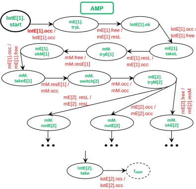
Figure A3. Agent automaton of AMP agent type.
The server view of the system is automatically converted to the agent view by the Dedan program. In the agent view, actions are grouped for individual agents. During the conversion, the type AMP is
split into two separate types AMP and AMP__1, due to different initial messages. Consequently, vector
elements AMP[1] and AMP[2] are renamed to separate agent variables AMP and AMP__1. The agent
view shows the system from the point of view of the AMP vehicles (Listing below). Fig. A3 presents
a fragment of the AMP agent type automaton.
1. agent: AMP (servers mE[2]:mE,mM:mM,lotE[2]:lotE,lotM:lotM), 2. actions {
3. {AMP.lotE[1].try, lotE[1].free} -> {AMP.mE[1].okL, lotE[1].res},
4. {AMP.lotE[1].ok, lotE[1].occ} -> {AMP.mE[1].takeL, lotE[1].free},
5. {AMP.lotE[1].start, lotE[1].occ} -> {AMP.mE[1].tryL, lotE[1].occ},
6. {AMP.lotE[1].take, lotE[1].res} -> {lotE[1].occ},
7. {AMP.lotE[2].try, lotE[2].free} -> {AMP.mE[2].okL, lotE[2].res},
8. {AMP.lotE[2].ok, lotE[2].occ} -> {AMP.mE[2].takeL, lotE[2].free},
10. {AMP.lotE[2].take, lotE[2].res} -> {lotE[2].occ},
11. <j=1..2> {AMP.lotM.try[j], lotM.free} -> {AMP.mM.okL[j], lotM.res[j]}, 12. <j=1..2> {AMP.lotM.ok[j], lotM.occ[j]} -> {AMP.mM.takeL[j], lotM.free}, 13. <j=1..2> {AMP.lotM.take[j], lotM.res[j]} -> {AMP.mM.tryL[j], lotM.occ[j]}, ...
Appendix B - Using DA3 in the Dedan program
The basic form used in Dedan program is IMDS, because it allows for automatic conversion between the server view and the agent view of a system. Yet, the specification in the form of a relation between pairs λ=((state,message),(state’,message’)) is exotic for the users. Therefore, an alternative input
form of DA3 automata is provided.
A system may be simulated over the global space of configurations (LTS), but it is also possible to simulate it in terms of S-DA3, as illustrated in Fig. 5. All of the automata in the system are displayed,
with input sets of pending messages under automata identifiers shown. The current states of the automata are blue.
A user can choose an automaton (Sprod in the example, the chosen automaton has white background and blue name), and then a list of transitions from the current state of the chosen automaton is displayed on the left (with enabled ones distinguished; it is only one transition in this case, and it is enabled). Next, the user may choose a transition from the enabled ones. In the example
it is only one transition enabled, leading from neutral to prod (with acceptance of doSth message
and issuing of put message to buf). If the user clicks an enabled transition, it is “executed” and a destination automaton of the message becomes current (buf in this case).
References
1. Daszczuk, W.B.: Specification and Verification in Integrated Model of Distributed Systems (IMDS). MDPI Comput. 7 (4), 1–26 (2018).
2. Baier, C., Katoen, J.-P.: Principles of Model Checking. MIT Press, Cambridge, MA (2008). ISBN 9780262026499
3. Schwarick, M.: MARCIE - Model Checking and Reachability Analysis Done EffiCIEntly. Eighth International Conference on Quantitative Evaluation of SysTems, Aachen, Germany, 5-8 Sept. 2011, pp. 91-100, IEEE (2013). doi: 10.1109/QEST.2011.19
4. Daszczuk, W.B.: Siphon-based deadlock detection in Integrated Model of Distributed Systems (IMDS). In: Federated Conference on Computer Science and Information Systems, 3rd Workshop on Constraint Programming and Operation Research Applications (CPORA’18), Poznań, Poland, 9-12 Sept. 2018. pp. 425–435. IEEE (2018). doi:10.15439/2018F114
5. Heiner, M., Schwarick, M., Wegener, J.-T.: Charlie – An Extensible Petri Net Analysis Tool. In: 36th International Conference, PETRI NETS 2015, Brussels, Belgium, 21-26 June 2015. pp. 200–211. Springer International Publishing, Cham, Switzerland (2015). doi:10.1007/978-3-319-19488-2_10
6. Holzmann, G.J.: The model checker SPIN. IEEE Trans. Softw. Eng. 23 (5), 279–295 (1997). doi:10.1109/32.588521
7. Cimatti, A., Clarke, E., Giunchiglia, F., Roveri, M.: NUSMV: A new symbolic model checker. Int. J. Softw. Tools Technol. Transf. 2 (4), 410–425 (2000). doi:10.1007/s100090050046
8. Behrmann, G., David, A., Larsen, K.G., Pettersson, P., Yi, W.: Developing UPPAAL over 15 years. Softw. Pract. Exp. 41 (2), 133–142 (2011). doi:10.1002/ spe.1006
9. Alur, R., Dill, D.L.: A theory of timed automata. Theor. Comput. Sci. 126 (2), 183–235 (1994). doi:10.1016/0304-3975(94)90010-8
10. Lanese, I., Montanari, U.: Hoare vs Milner: Comparing Synchronizations in a Graphical Framework With Mobility. Electron. Notes Theor. Comput. Sci. 154 (2), 55–72 (2006). doi:10.1016/j.entcs.2005.03.032 11. May, D.: OCCAM. ACM SIGPLAN Not. 18 (4), 69–79 (1983). doi:10.1145/ 948176.948183
12. Reniers, M.A., Willemse, T.A.C.: Folk Theorems on the Correspondence between State-Based and Event-Based Systems. In: 37th Conference on Current Trends in Theory and Practice of Computer Science, Nový Smokovec, Slovakia, 22-28 Jan. 2011, LNCS vol. 6543. pp. 494–505. Springer-Verlag, Berlin Heidelberg (2011). doi:10.1007/978-3-642-18381-2_41
Branching Time Properties. Fundam. Informaticae. 43 (1-4), 245–267 (2000). doi:10.3233/FI-2000-43123413
14. Daszczuk, W.B.: Deadlock Detection Examples: The Dedan Environment at Work. In: Integrated Model of Distributed Systems, SCI vol. 817, pp. 53–85. Springer Nature, Cham, Switzerland (2020). doi: 10.1007/978-3-030-12835-7_5
15. Daszczuk, W.B.: Asynchronous Specification of Production Cell Benchmark in Integrated Model of Distributed Systems. In: Bembenik, R., Skonieczny, L., Protaziuk, G., Kryszkiewicz, M., and Rybinski, H. (eds.) 23rd International Symposium on Methodologies for Intelligent Systems, ISMIS 2017, Warsaw, Poland, 26-29 June 2017, Studies in Big Data, vol. 40. pp. 115–129. Springer International Publishing, Cham, Switzerland (2019). doi: 10.1007/978-3-319-77604-0_9
16. Czejdo, B., Bhattacharya, S., Baszun, M., Daszczuk, W.B.: Improving Resilience of Autonomous Moving Platforms by real-time analysis of their Cooperation. Autobusy-TEST. 17 (6), 1294–1301 (2016). arXiv:1705.04263
17. UML, Available online: http://www.uml.org/ (accessed 6.12.2019)
18. Zielonka, W.: Notes on finite asynchronous automata. RAIRO - Theor. Informatics Appl. 21 (2), 99–135 (1987). doi: 10.1051/ita/1987210200991
19. Krishnan, P.: Distributed Timed Automata. Electron. Notes Theor. Comput. Sci. 28, 5–21 (2000). doi:10.1016/S1571-0661(05)80627-9
20. Muscholl, A.: Automated Synthesis of Distributed Controllers. In: Automata, Languages, and Programming - 42nd International Colloquium, {ICALP} 2015, Kyoto, Japan, 6-10 July 2015, Part {II}. pp. 11–27 (2015). doi:10.1007/978-3-662-47666-6_ 2
21. Diekert, V., Muscholl, A.: On Distributed Monitoring of Asynchronous Systems. In: 19th International Workshop on Logic, Language, Information and Computation, WoLLIC 2012, Buenos Aires, Argentina, 3-6 Sept. 2012. pp. 70–84. Springer, Berlin Heidelberg (2012). doi:10.1007/978-3-642-32621-9_5
22. Mukund, M.: Automata on Distributed Alphabets. In: Modern Applications of Automata Theory. pp. 257–288. Co-Published with Indian Institute of Science (IISc), Bangalore, India (2012). doi:10.1142/9789814271059_0009
23. Sandholm, A.B., Schwartzbach, M.I.: Distributed Safety Controllers for Web Services. BRICS Rep. Ser. 4 (47), (1997). doi:10.7146/brics.v4i47.19268
24. Brim, L., Černá, I., Moravec, P., Šimša, J.: How to Order Vertices for Distributed LTL Model-Checking Based on Accepting Predecessors. Electron. Notes Theor. Comput. Sci. 135 (2), 3–18 (2006). doi:10.1016/j.entcs.2005.10.015
25. Bollig, B., Leucker, M.: Message-Passing Automata Are Expressively Equivalent to EMSO Logic. In: 15th International Conference CONCUR 2004 - Concurrency Theory, London, UK, 31 Aug. - 3 Sept. 2004. pp. 146–160. Springer, Berlin Heidelberg (2004). doi:10.1007/978-3-540-28644-8_10
26. Bollig, B., Leucker, M.: A Hierarchy of Implementable MSC Languages. In: Formal Techniques for Networked and Distributed Systems - FORTE 2005, Taipei, Taiwan, 2-5 Oct. 2005. pp. 53–67. Springer, Berlin Heidelberg (2005). doi:10.1007/11562436_6
27. Balan, M.S.: Serializing the Parallelism in Parallel Communicating Pushdown Automata Systems. Electron. Proc. Theor. Comput. Sci. 3, 59–68 (2009). doi: 10.4204/EPTCS.3.5
28. Enea, C., Habermehl, P., Inverso, O., Parlato, G.: On the Path-Width of Integer Linear Programming. Electron. Proc. Theor. Comput. Sci. 161, 74–87 (2014). doi:10.4204/EPTCS.161.9
29. Madhusudan, P., Parlato, G.: The tree width of auxiliary storage. In: Proceedings of the 38th annual ACM SIGPLAN-SIGACT symposium on Principles of programming languages - POPL ’11, Austin, TX, 26-28 Jan. 2011. pp. 283–294. ACM Press, New York, NY (2011). . doi:10.1016/j.entcs.2005.03.032. 30. Huguet, S., Petit, A.: Modular constructions of distributing automata. In: Mathematical Foundations of
Computer Science 1995, 20th International Symposium, MFCS’95, Prague, Czech Republic, 28 Aug. - 1 Sept. 1995. pp. 467–478. Springer, Berlin Heidelberg (1995). doi:10.1007/3-540-60246-1_152
31. Petit, A.: Recognizable trace languages, distributed automata and the distribution problem. Acta Inform. 30 (1), 89–101 (1993). doi:10.1007/BF01200264
32. Krithivasan, K., Ramanujan, A.: On The Power of Distributed Bottom-up Tree Automata. Int. J. Adv. Comput. Sci. 3 (04), 184–190 (2013). Available online: http://worldcomp-proceedings.com/proc/p2011/FCS2998.pdf (accessed 6.12.2019)
In: Ben Ayed, R. and Djemame, K. (eds.) Second international conference on Verification and Evaluation of Computer and Communication Systems VECoS’08, Leeds, UK , 2-3 July 2008. pp. 38–49. British
Computer Society, Swinton, UK (2008). Available online:
https://www.researchgate.net/publication/254361167_A_Comparison_of_Distributed_Test_Generation _Techniques (accessed 6.12.2019)
34. Dick, G., Yao, X.: Model representation and cooperative coevolution for finite-state machine evolution. In: 2014 IEEE Congress on Evolutionary Computation (CEC), Beijing, China, 6-11 July 2014. pp. 2700– 2707. IEEE, New York, NY (2014). doi:10.1109/ CEC.2014.6900622