R E S E A R C H
Open Access
Low-complexity high-throughput decoding
architecture for convolutional codes
Ran Xu
1*, Kevin Morris
1, Graeme Woodward
2and Taskin Kocak
3Abstract
Sequential decoding can achieve a very low computational complexity and short decoding delay when the signal-to-noise ratio (SNR) is relatively high. In this article, a low-complexity high-throughput decoding architecture based on a sequential decoding algorithm is proposed for convolutional codes. Parallel Fano decoders are scheduled to the codewords in parallel input buffers according to buffer occupancy, so that the processing capabilities of the Fano decoders can be fully utilized, resulting in high decoding throughput. A discrete time Markov chain (DTMC) model is proposed to analyze the decoding architecture. The relationship between the input data rate, the clock speed of the decoder and the input buffer size can be easily established via the DTMC model. Different scheduling schemes and decoding modes are proposed and compared. The novel high-throughput decoding architecture is shown to incur 3-10% of the computational complexity of Viterbi decoding at a relatively high SNR.
Keywords:architecture, convolutional code, Fano algorithm, high-throughput decoding, scheduling, sequential decoding, WirelessHD
1 Introduction
The 57-64 GHz unlicensed bandwidth around 60 GHz can accommodate multi-gigabits per second (multi-Gbps) wireless transmission in a short range. There are several standards for 60 GHz systems, such as lessHD [1] and IEEE 802.15.3c [2,3]. In both Wire-lessHD and the AV PHY mode in IEEE 802.15.3c, a concatenated FEC scheme is used with a RS code as the outer code and a convolutional code as the inner code. In order to achieve the target decoding throughput at multi-Gbps, parallel convolutional encoding has been adopted by the transmitter baseband design in both standards. It is straightforward to use parallel Viterbi decoding in the receiver baseband. However, it has been shown in [4,5] that parallel Viterbi decoders in the receiver baseband result in massive hardware complexity and power consumption. The problem will become more severe if a higher decoding throughput is targeted (i.e., 10 Gbps) for a battery powered user terminal in the future [6]. Hence it is desirable to find a
low-complexity high-throughput decoding method for con-volutional codes in such systems.
The Viterbi algorithm (VA) achieves maximum likeli-hood decoding for convolutional codes [7]. The VA is a breadth-first, exhaustive search approach based on the trellis diagram. Sequential decoding is another method of convolutional decoding and is a depth-first, non-exhaustive searching approach based on the tree dia-gram. It only explores partial paths locally in the code tree, so it has sub-optimal decoding performance and its computational complexity varies with SNR. There are two main types of sequential decoding algorithms which are known as the Stack algorithm [8] and the Fano algo-rithm [9,10]. Because the Fano algoalgo-rithm has low sto-rage and sorting requirements, it can achieve higher decoding throughput compared to the Stack algorithm. Only the Fano algorithm is considered in this article. Sequential decoding is not widely used in real systems due to the excessive computations and long decoding delay when the SNR is low. However, if a relatively high SNR can be achieved (e.g., for a very short range and/or via beamforming) or required for some applications (e. g., HD video streaming), sequential decoding will on average incur a very low computational complexity and
* Correspondence: [email protected]
1
Centre for Communications Research, Department of Electrical & Electronic Engineering, University of Bristol, Bristol, UK
Full list of author information is available at the end of the article
short decoding delay, which results in a high decoding throughput.
In this article, a novel low-complexity high-throughput decoding architecture based on parallel Fano algorithm decoding with scheduling is proposed. Different schedul-ing schemes and decodschedul-ing modes are investigated. A discrete time Markov chain (DTMC) is introduced to model the proposed architecture to establish the rela-tionship between input data rate, input buffer size, and clock speed of the decoders. The trade-offs between error rate, computational complexity, scheduling schemes and decoding modes are studied. It will be shown that the high-throughput decoding architecture can achieve a much lower computational complexity compared to the Viterbi decoding with a similar error rate performance. The rest of the article is organized as follows. First, the unidirectional Fano algorithm (UFA) and bidirectional Fano algorithm (BFA) are reviewed in Section 2. The novel parallel Fano decoding with sche-duling architecture is proposed in Section 3. Different scheduling schemes and decoding modes are also pro-posed in this section. The DTMC based modeling is applied to the decoding architecture in Section 4. Simu-lation results are given in Section 5, and the conclusions are drawn in Section 6.
2 Unidirectional Fano algorithm and bidirectional Fano algorithm
In the conventional unidirectional Fano algorithm, the decoder starts decoding from the initial state zero (or origin node). During each iteration of the algorithm, the decoder may move forward (increase depth within the tree), move backward (reduce depth), or stay at the cur-rent tree depth. The decision is made based on the comparison between the threshold value and the path metric. If a forward movement is made, the threshold value needs to be tightened. If the decoder cannot move forward or backward, the threshold value needs to be loosened. A detailed flowchart of the UFA can be found in [11].
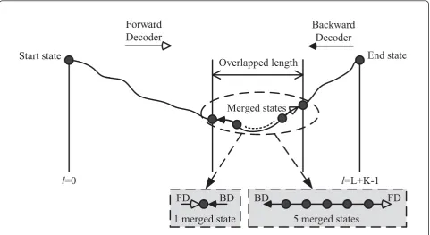
A bidirectional Fano algorithm was proposed in [12]. Both the forward decoder (FD) and backward decoder (BD) start decoding from the known state zero and per-form decoding in the forward and backward direction in parallel as shown in Figure 1. The decoding will finish if the FD and the BD merge somewhere in the code tree. Otherwise, if the FD and the BD cannot merge, the decoding will finish when either of them reaches the other end of the code tree. Merging means that the FD and the BD have the same encoder state and the same level within the codeword. A simple merging condition requires the FD and the BD have one merged state as shown in the shaded box on the left. A more rigorous merging condition requires the FD and the BD to have
more than one merged state (e.g., 5 merged states) as shown in the shaded box on the right. By increasing the number of merged states (NMS), the probability that the FD and the BD to decode on the same path can be increased, resulting in an improved error rate perfor-mance. However, this is at the cost of higher computa-tional effort. This trade-off has been discussed in [13]. In this article, the simple merging condition (NMS = 1) is adopted by the BFA.
The simulated complementary cumulative distribu-tions of computational complexity of the UFA, the BFA and the VA are compared in Figure 2 at different SNR values. The computational complexity is measured by the number of branch metric calculations (BMC). It can be seen that as the SNR increases, the computational complexity and variability of the UFA and the BFA reduce. However, the computational complexity of the VA has a constant value which does not change with the SNR. Additionally, the BFA can achieve a lower computational complexity and variability compared to the UFA, which is more pronounced at a lower SNR. 3 Parallel Fano decoding with scheduling
3.1 Architecture
can also be used to decode very long constraint length convolutional codes which may be infeasible for the Viterbi algorithm to decode.
A reference receiver baseband designafor the Wire-lessHD and IEEE 802.15.3c standards is shown in Figure 4. The building blocks operate in reverse compared to the corresponding building blocks at the Tx. There are eight parallel convolutional decoders, and the VA can be implemented in each of them. However, it is one of the most power and hardware intensive blocks in the Rx baseband. The system operates in indoor and short range environments, so it is possible that there is a line-of-sight (LOS) path between the Tx and the Rx which enables a relatively high SNR at the Rx. Even if the LOS component is not available, the adaptive antenna beam-forming technique can still guarantee a relatively high SNR at the Rx. Additionally, the Tx and the Rx are quasi-static, which means the SNR is roughly constant. All these facts make sequential decoding algorithm an attractive approach for high-throughput convolutional decoding.
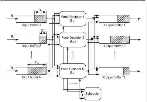
In Figure 5 there areNparallel Fano decoders each with a finite input buffer accommo-dating up toBcodewords. The supported input data rate of each buffer is assumed to beRdinformation bits per second. The total supported data rate or average decoding throughput will beN·Rd. This parallel Fano decoding system can be treated as a
parallel queuing system, in which the parallel input buffers are the queues and the parallel Fano decoders are the ser-vers. Due to the variable computational efforts of the Fano decoders, the input buffer occupancies (Q1,...,QN) vary from each other as shown in Figure 5. If the Fano deco-ders can be scheduled to decode the codewords in differ-ent input buffers, the utilization of the Fano decoders can be increased, resulting in a higher decoding throughput. For example, if a Fano decoderFmfinishes decoding one
codeword and its input buffer occupancy is lower than that of another input buffer, i.e.,Bn, it is possible to
sche-dule the decoderFmto help decoding another codeword
in the input bufferBn, thus to reduceQnto avoid potential buffer overflow or frame erasure. In order to realize this, a scheduler is introduced which can allocate the Fano deco-ders to the input buffers dynamically as shown in Figure 5. Each Fano decoder also needs to connect to all the input and output buffers. The scheduler is invoked when a deco-der finishes decoding one codeword. It then allocates the decoder to an input buffer according to some scheduling scheme. The allocation of the decoders to the input buf-fers can be achieved by changing the connectivities between the input buffers and the decoders and those between the decoders and the output buffers.
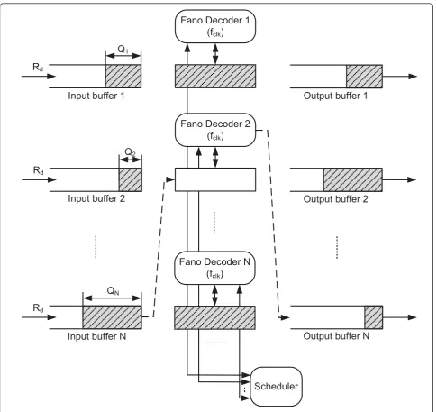
For ease of analysis and modeling, an equivalent archi-tecture is proposed in Figure 6. Each Fano decoder has a buffer which can hold one codeword, and the codeword
l
=0
l
=L+K-1
Merged states
Start state
End state
Forward
Decoder
Backward
Decoder
Overlapped length
1 merged state
5 merged states
FD
BD
BD
FD
in this buffer may come from any of the parallel long input buffers whose size isB - 1. When a decoderFm
finishes decoding the codeword in its buffer, the buffer is cleared and updated with a new codeword from a
long input buffer according to some scheduling scheme. For example, as shown in Figure 6, when the decoder
F2finishes decoding the codeword in its buffer, the scheduler selects the long input bufferBNaccording to
102 103 104 105 106 10−4
10−3 10−2 10−1 100
BMC
Pr(C>X)
Computational complexity distribution
UFA BFA VA
5dB 6dB
4dB 3dB
UFA
BFA VA
Figure 2Computational complexity distributions of the UFA, the BFA and the VA in the AWGN channel.
m
1m
2m
3m
4m
5m
6Input bits
X
Y
Z
some scheduling scheme. If its occupancy is greater or equal to one codeword lengthLf, i.e.,QN≥Lf, the buffer ofF2is updated with a new codeword fromBN and the
occupancy ofBNis reduced QN=QN - Lf; otherwise if QN<Lf, a“virtual link”is setup betweenBNandF2until QN≥Lf. The difference between Figures 5 and 6 is that
the parallel long input buffers are not necessarily attached to the Fano decoders in the equivalent archi-tecture, which makes the understanding of the system much easier.
When an input buffer Bnis about to overflow, the
scheduler compares the computational efforts of all the
De-scrambler
RS Decoder
RS Decoder
Outer De-interleaver Outer De-interleaver
Convolutional Decoder
Mux 4:1 Mux 4:1
Convolutional Decoder Convolutional
Decoder Convolutional
Decoder
Bit De-interleaver
Demux 1:8
Other Baseband
Blocks Rx
Beam-forming
Figure 4Receiver reference implementation block diagram.
Fano Decoder 1 (fclk) Rd
Fano Decoder N (fclk) Rd
Fano Decoder 2 (fclk) Rd
Scheduler Input buffer 1
Input buffer 2
Input buffer N
Output buffer 1
Output buffer 2
Output buffer N Q1
Q2
QN
decoders and erases the codeword of the decoderFmif
it has consumed the highest computational effort among all the decoders. After the codeword of the decoderFmis erased, one codeword in the input buffer Bnis scheduled to the decoder Fmand the occupancy
of the input bufferBnis reduced Qn=Qn- Lf.
The number of decodersMis assumed to be the same as the number of input buffersNin Figures 5 and 6 (i.e., M = N) for ease of illustration. However, it will be shown in Section 5 that a higher number of decoders may be required to achieve a target decoding through-put (i.e.,M>N).
3.2 Scheduling schemes
When a decoder finishes decoding a codeword, the scheduler needs to decide which input buffer the deco-der should serve next. It has been discussed in [18-20] that serving the longest queue first (LQF) can help mak-ing the parallel queues (or input buffers) the most balanced or stable, thus maximising the input data rate Rd. The scheduled decoders serving the longest queue first is considered to be one of the best scheduling schemes in the proposed architecture in terms of achieving a high decoding throughput.
The LQF scheme needs to compare the input buffer occupancy values. Other simpler scheduling schemes
Fano Decoder 1
(f
clk)
R
dR
dR
dScheduler
Input buffer 1
Input buffer 2
Input buffer N
Output buffer 1
Output buffer 2
Output buffer N
Q
1Q
2Q
NFano Decoder 2
(f
clk)
Fano Decoder N
(f
clk)
can be employed to reduce the computational and hard-ware complexity of the scheduler. One possible schedul-ing scheme is to randomly select the input buffer, which is named the RDM scheme. Another scheduling scheme is to group the parallel input buffers and decoders, such that each decoder can only be scheduled to the input buffers within the same group. The decoders in the same group are scheduled according to the LQF scheme. This is known as the static scheduling scheme or the STC scheme. In this article, each group is assumed to have two input buffers and two UFA deco-ders. Compared to the LQF scheme, the STC scheme can help reducing the need for multi-port memories and high fan-out multiplexers. It can also simplify the design of the scheduler and the connections between the input buffers and the decoders.
3.3 PUFAS mode and PBFAS mode
When a decoder Fmfinishes decoding a codeword, it
can be scheduled to decode a new codeword from one of the input buffers, or it can be scheduled to help another decoder Fm which has already been working
on a whole codeword. The scheduled decoder Fmcan
decode from the end state zero of this codeword, which makes Fmand Fm decode the same codeword in the
BFA mode. These two modes are known as the parallel unidirectional Fano algorithm decoding with scheduling (PUFAS) mode and the parallel bidirectional Fano algo-rithm decoding with scheduling (PBFAS) mode, respec-tively. It has been shown in [12,13] that the decoding throughput of a BFA decoder is at least two times of a UFA decoder (DBFA≥2DUFA) due to the parallel proces-sing between the FD and the BD and also due to the computational effort reduction achieved by the BFA. As a result, if there are MUFA decoders among which any two can decode in the BFA mode, the decoding throughput can be improved by forming ⌊M/2⌋ BFA decoders. In this case, there will be⌊M/2⌋parallel BFA decoders which can be scheduled in the architecture. 4 DTMC based modeling
In the proposed parallel Fano decoding with scheduling architecture, the total number of codewords can be writ-ten:
Ntotal=Ndecoded+Nerased, (1)
where Ndecodedis the number of decoded codewords and Nerasedis the number of erased codewords due to buffer overflow. A metric called blocking probability (PB) is defined as:
PB= Nerased
Ntotal
= Nerased
Ndecoded+Nerased
, (2)
wherePBis similar to the frame error rate (PF) caused by undetected errors. In designing the system, the input data rateRd(in bps), the clock speed of each Fano deco-der fclk (in Hz) and the input buffer size B (in code-words) need to be chosen properly to ensure that:
PBPF. (3)
In this article,PB=0.01 × PFis adopted as the target blocking probability (Ptarget). The relationship between Rd,fclkandBcan be found via simulation. Another way to analyze the architecture is to model it based on queu-ing theory.
4.1 DTMC based modeling on single UFA/BFA
A single UFA/BFA decoder with a finite input buffer can be treated as a D/G/1/Bqueue [21], in which D means that the input data rate is deterministic,Gmeans that the decoding time is generic, 1 means that there is one decoder and B is the number of codewords the input buffer can hold. The state of the Fano decoder is represented by the input buffer occupancy or queue length when a codeword just finishes decoding, which is measured in terms of branches or information bits stored in the buffer.Q(n) and Q(n+ 1) have the follow-ing relationship:
Q(n+ 1) =Q(n) + [Ts(n)·Rd−Lf], (4)
where Q(n + 1) is the input buffer occupancy when the nth codeword just finishes decoding, Ts(n) is the decoding time of thenth codeword by the Fano decoder andLfis the length of a codeword in terms of branches or information bits. [x] denotes the operation to get the nearest integer to x. The speed factor of the Fano deco-der is defined as the ratio betweenfclkandRd:
μ= fclk
Rd
. (5)
Iffclkis normalized to 1, Equation (4) can be changed to:
Q(n+ 1) =Q(n) + [Ts(n)
μ −Lf]. (6)
analysis since its closed form expression is intractable. The difference betweenQ(n+ 1) andQ(n) is defined as:
(n) =Q(n+ 1)−Q(n) = [Ts(n)
μ −Lf]. (7)
The total number of states of the input buffer with sizeBis:
=B·Lf. (8)
The state transition probability matrix of the input buffer is:
where Pij is the state transition probability from Sito Sjwhich can be calculated as follows:
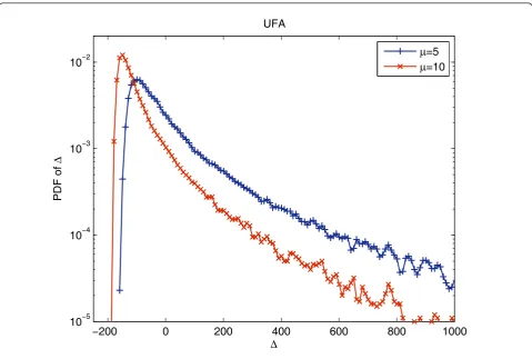
Pij= The value of p+wcan be estimated from the simulated distribution of Ts, which is shown in Figure 7 for the UFA with different speed factors at Eb/N0 = 4dB. It should be noted that a bad codeword may incur unbounded decoding time for a Fano decoder and it is common to erase this codeword. This case corresponds to j = Ω in Equations (9) and (10). The initial state probability (n= 0) of the input buffer is:
π(0) = (π1(0),π2(0), ...,π(0)) = (1, 0, ..., 0), (11) where πω(n) is the probability that the input buffer is in stateSωat timen. The steady state probability of the input buffer is then:
= lim
n→∞π(n) = limn→∞π(0)·P n
T. (12)
Hence, the blocking probability of the decoder can be calculated by:
where ∏(i) is the steady state probability that the input buffer is in stateSiandp+−i= Pr( > −i).
4.2 Extension to PUFAS/PBFAS-LQF
When scheduling is involved, it is difficult to apply DTMC based modeling since the parallel queues behave in a very complex way. However, if the LQF scheduling scheme is used, the proposed decoding architecture can be modelled by the DTMC in an approximate way. If there are M Fano decoders working in parallel with each running atfclkand the LQF scheduling scheme is used, the M Fano decoders can be fully utilized to decode the codewords in the Ninput buffers. Since the M Fano decoders and theNinput buffers are identical to each other, the system is totally symmetric and can be treated as a faster Fano decoder with the clock speed of fclk =M·fclkworking on each input buffer with the
The state transition probability matrixPT,ican be cal-culated based on the distribution of Δi, and Equations (8)-(13) can still be applied to the PUFAS/PBFAS-LQF. The validation of the proposed DTMC model will be confirmed by the simulation results shown in the fol-lowing section.
5 Simulation results
5.1 Comparison between different scheduling schemes
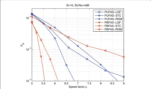
The performance of different scheduling schemes is compared by simulation in Figure 8. The SNR was set asEb/N0= 4 dB which corresponds to the target block-ing probability ofPtarget= 10-3. In both the PUFAS and the PBFAS, the LQF scheduling scheme has the best performance. In the PUFAS the RDM scheme has a bet-ter performance compared to the STC scheme, while in the PBFAS the RDM scheme has the worst performance compared to all the other schemes. This is because when the RDM scheme is employed in the PBFAS, a BFA decoder may become idle if it randomly selects a low occupancy input buffer. But the wrong selection by the RDM scheme in the PUFAS may make only one UFA decoder idle. As a result, the RDM scheme can be used in the PUFAS and the STC scheme can be used in the PBFAS to reduce the complexity of the scheduler. However, since the complexity added by the LQF sche-duler to the parallel decoders is minimal, it is favoured in terms of achieving a higher decoding throughput.
5.2 Validation of the DTMC model
The semi-analytical resultsbare compared with the simu-lation results to validate the DTMC model. It can be seen
from Figure 9 that the semi-analytical results are quite close to the simulation results, which indicates the accu-racy of the proposed DTMC model. The working speed factor of the parallel unidirectional Fano algorithm decod-ing without scheduldecod-ing (PUFA) is aboutμ= 17 which can be reduced toμ= 7 and μ= 5.6 if the LQF scheduling scheme is performed in the PUFAS and in the PBFAS, respectively. The corresponding decoding throughput improvements are 140% and 200%, respectively.
It has been found that the proposed DTMC based modeling on the PUFAS-LQF and PBFAS-LQF is ideal when the input buffer size B is large enough (i.e.,B ≥ 5). The accuracy of the model degrades asBgets smal-ler. However, a very short input buffer will not be adopted according to the trade-off between area and decoding throughput as discussed in [21]. Additionally, it has also been found that the accuracy of the model does not depend on the relationship betweenM andN (i.e.,M>N, M=Nor M<N) as long as the input buffer size is large enough.
5.3 Number of parallel Fano decoders
Figure 10 shows the relationship between the number of parallel Fano decoders Mand the working speed factors
−200 0 200 400 600 800 1000
10−5 10−4 10−3 10−2
PDF of
UFA
=5
=10
5 5.5 6 6.5 7 7.5 8 8.5 9 10−3
10−2 10−1
Speed factor
P B
B=10, Eb/No=4dB
PUFAS−LQF PUFAS−STC PUFAS−RDM PBFAS−LQF PBFAS−STC PBFAS−RDM
Figure 8Blocking probabilityPBversus speed factorμfor different scheduling schemes with the number of input buffersN= 8 and
the number of parallel Fano decodersM= 8 atEb/N0= 4 dB.
4 6 8 10 12 14 16
10−3 10−2 10−1
Speed factor
P B
B=10, Eb/No=4dB
PUFA, semi−analytical PUFA, simulation
PUFAS−LQF, semi−analytical PUFAS−LQF, simulation PBFAS−LQF, semi−analytical PBFAS−LQF, simulation
PUFA PUFAS−LQF
PBFAS−LQF
Figure 9Blocking probabilityPBversus speed factorμfor the PUFA, the PUFAS-LQF and the PBFAS-LQF with the number of input
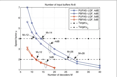
μfor both the PUFAS-LQF and the PBFAS-LQF atEb/ N0= 4dB and 5dB, respectively. This relationship can be easily established by the proposed DTMC model.
If the target decoding throughput is Dtarget= 1 Gbps and the clock speed of the Fano decoder is fclk = 500 MHz, the supported input data rate will beRd =Dtarget/ N= 125 Mbps for N= 8 input buffers and the target speed factor will beμ1 =fclk/Rd= 4. It can be seen from Figure 10 that the required number of decoders is M= 14 for the PUFAS-LQF andM= 12 for the PBFAS-LQF at Eb/N0 = 4dB. Two decoders can be saved if the PBFAS-LQF is adopted compared to the PUFAS-LQF for the same decoding throughput.
It can also be seen from Figure 10 that the decoding throughput can be improved as SNR increases for the same number of decoders. As a result, some of the decoders can be dynamically turned off as SNR increases for the same decoding throughput, though a large number of decoders may be required to support a low SNR. For example, if the target decoding through-put increases toDtarget= 2 Gbps and the clock speed of the Fano decoder is still fclk = 500 MHz, the target speed factor will be μ2 = 2. It can be seen from Figure 10 that the required number of decoders isM = 28 for
the PUFAS-LQF andM = 26 for the PBFAS-LQF atEb/ N0 = 4dB which can be reduced to only M = 12 if the SNR increases to 5dB. In this case, more than half of the decoders can be turned off to reduce the power con-sumption of the decoding architecture.
5.4 Error rate performance and computational complexity
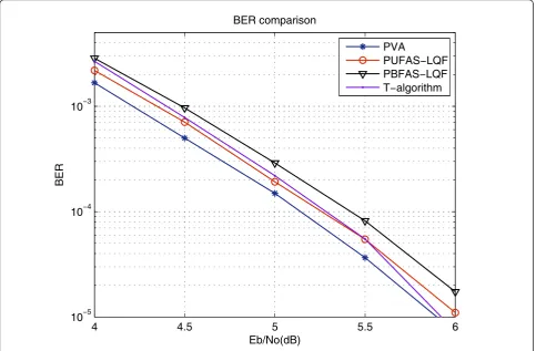
The proposed parallel Fano decoding with scheduling is compared with the parallel Fano decoding without sche-duling and the parallel Viterbi algorithm decoding (PVA) in terms of bit-error-rate (BER) and computa-tional complexity. As discussed in [24-26], the state-of-the-art low power Viterbi decoders based on theT -algo-rithm [27] can also achieve a reduced computational complexity at a high SNR with a minimal penalty in coding gain, so its performance is also included for comparison. It can be seen in Figure 11 that the PVA has the best BER performance. There is about 0.1dB penalty in coding gain at BER = 10-4 by using the PUFAS-LQF. The PBFAS-LQF has the worst perfor-mance and there is about 0.25 dB coding gain loss com-pared to the PVA. The T-algorithm has been tuned to achieve similar BER performance by setting the discard-ing thresholdT= 5.
5 10 15 20 25 30 35 40 1
2 3 4 5 6 7
Number of decoders M
Speed factor
Number of input buffers N=8
PUFAS−LQF, 4dB PBFAS−LQF, 4dB PUFAS−LQF, 5dB PBFAS−LQF, 5dB Target 1
Target 2
M=14 M=12
M=28 M=26
M=12
5dB 4dB
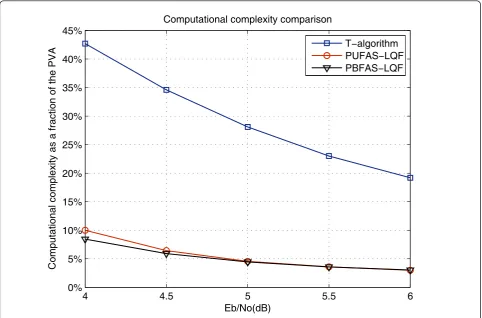
The computational complexity measured by the num-ber of branch metric calculations is compared in Figure 12. Each BMC corresponds to one node extension in the code tree or one state update in the trellis diagram. Each state update in the VA involves an ACS operation, which has the similar computational complexity as one node extension in the UFA or BFA. This quantity has been widely used in the literature to compare Viterbi decoding and sequential decoding in terms of computa-tional complexity [28,29]. The computacomputa-tional complexity of the PUFAS-LQF to decode one codeword is:
CPUFAS=CUFA+CS, (16)
whereCUFA is the computational complexity of the UFA decoder andCS is the computational complexity of the LQF scheduler. It is known that CUFA ≥ Lf= 206 BMC and CS is onlyN- 1 = 7 times input buffer occu-pancy values comparisons. As a result, the computa-tional complexity of the PUFAS-LQF to decode one codeword is CPUFAS ≈ CUFA. Similarly, the computa-tional complexity of the PBFAS-LQF to decode one codeword is:
CPBFAS≈CBFA=CFD+CBD, (17)
where CFD is the number of BMC to decode one codeword in the forward direction andCBDis the num-ber of BMC in the backward direction. The computa-tional complexity of the PVA to decode one codeword has a fixed value:
CPVA= 2K−1×Lf. (18)
The distributions of CUFA, CBFA, and CVAat different SNR can be found in Figure 2.
It can be seen that the proposed decoding architecture consumes a much lower computational complexity com-pared to the PVA. For example at Eb/N0 = 4 dB, the computational complexity of the PUFAS-LQF is only 10% of the PVA and it reduces to 3% at 6 dB. Addition-ally, the computational complexity of the PBFAS-LQF is lower than that of the PUFAS-LQF at a lower SNR, but they become very similar as SNR increases. This is because at a high SNR, the computational complexity reduction achieved by the BFA compared to the UFA becomes minimal. Since there is a very limited
4 4.5 5 5.5 6
10−5 10−4 10−3
Eb/No(dB)
BER
BER comparison
PVA
PUFAS−LQF PBFAS−LQF T−algorithm
improvement on decoding throughput and computa-tional complexity by using the PBFAS-LQF compared to the PUFAS-LQF at a high SNR, the PUFAS-LQF is favored due to its better BER performance. It can also be seen from Figures 11 and 12 that with a similar BER performance as the PUFAS-LQF and the PBFAS-LQF the T-algorithm cannot achieve the same low computa-tional complexity.
6 Conclusions
This article considered the application of sequential decoding algorithm in high-throughput wireless commu-nication systems. A novel architecture based on parallel Fano algorithm decoding with scheduling was proposed. Due to the scheduling of the Fano decoders according to the input buffer occupancy, a high decoding through-put can be achieved by the proposed architecture. Dif-ferent scheduling schemes and decoding modes were proposed and compared. It was shown that the PBFAS-LQF scheme could achieve the highest decoding throughput. A DTMC model was proposed for the decoding architecture. The relationship between the input data rate, the clock speed of the decoder and the input buffer size can be easily established via the DTMC
model. The model was validated by simulation and uti-lized to determine the number of decoders required for a target decoding throughput. It was shown that the novel high-throughput decoding architecture requires 3-10% of the computational complexity of the Viterbi decoding with a similar error rate performance. This novel architecture can be employed in high-throughput systems such as 60 GHz systems to achieve energy effi-cient low-complexity convolutional codes decoding. Endnotes
a
The standard does not specify the Rx design. Only the Tx design is given. bSince the distribution of Ts is obtained by simulation, the DTMC based results are referred to as semi-analytical.
Acknowledgements
The authors would like to thank the Telecommunications Research Laboratory (TRL) of Toshiba Research Europe Ltd and its directors for supporting this study.
Author details
1Centre for Communications Research, Department of Electrical & Electronic
Engineering, University of Bristol, Bristol, UK2Wireless Research Centre, College of Engineering, University of Canterbury, Christchurch, New Zealand
4 4.5 5 5.5 6
0% 5% 10% 15% 20% 25% 30% 35% 40% 45%
Eb/No(dB)
Computational complexity as a fraction of the PVA
Computational complexity comparison
T−algorithm PUFAS−LQF PBFAS−LQF
3Department of Computer Engineering, Bahcesehir University, Istanbul,
Turkey
Competing interests
The authors declare that they have no competing interests.
Received: 23 August 2011 Accepted: 23 April 2012 Published: 23 April 2012
References
1. WirelessHD Specification Version 1.1 Overview, http://www.wirelesshd.org/ pdfs/WirelessHD-Specification-Overview-v1.1May2010.pdf
2. IEEE Standard for Information technology-Telecommunications and information exchange between systems-Local and metropolitan area networks-Specific requirements. Part 15.3: Wireless Medium Access Control (MAC) and Physical Layer (PHY) Specifications for High Rate Wireless Personal Area Networks (WPANs) Amendment 2: Millimeter-wave-based Alternative Physical Layer Extension. IEEE Std 802.15.3c-2009 (Amendment to IEEE Std 802.15.3-2003) (2009)
3. IEEE 802.15 WPAN Task Group 3c (TG3c) Millimeter Wave Alternative PHY http://www.ieee802.org/15/pub/TG3c.html
4. S Kato, H Harada, R Funada, T Baykas, C Sam, W Junyi, M Rahman, Single carrier transmission for multi-gigabit 60-GHz WPAN systems. IEEE J Sel Areas Commun.27(8), 1466–1478 (2009)
5. M Marinkovic, M Piz, C Choi, G Panic, M Ehrig, E Grass, Performance evaluation of channel coding for Gbps 60-GHz OFDM-based wireless communications, inIEEE 21st International Symposium on Personal Indoor and Mobile Radio Communications (PIMRC), Istanbul, Turkey, pp. 994–998 (2010)
6. G Fettweis, F Guderian, S Krone, Entering the path towards terabit/s wireless links, inDesign, Automation and Test in Europe Conference and Exhibition (DATE), Grenoble, France, pp. 1–6 (2011)
7. A Viterbi, Error bounds for convolutional codes and an asymptotically optimum decoding algorithm. IEEE Trans Inf Theory.13(2), 260–269 (1967) 8. F Jelinek, Fast sequential decoding algorithm using a stack. IBM J Res
Develop.13(6), 675–685 (1969)
9. R Fano, A heuristic discussion of probabilistic decoding. IEEE Trans Inf Theory.9(2), 64–74 (1963). doi:10.1109/TIT.1963.1057827
10. W Pan, A Ortega, Adaptive computation control of variable complexity Fano decoders. IEEE Trans Commun.57(6), 1556–1559 (2009) 11. S Lin, D Costello,Error Control Coding: Fundamentals and Applications,
(Pearson Prentice-Hall, Upper Saddle River, NJ, 2004)
12. R Xu, T Kocak, G Woodward, K Morris, C Dolwin, Bidirectional Fano algorithm for high throughput sequential decoding, inIEEE 20th International Symposium on Personal, Indoor and Mobile Radio Communications (PIMRC), Tokyo, Japan, pp. 1809–1813 (2009) 13. R Xu, T Kocak, G Woodward, K Morris, Throughput improvement on
bidirectional Fano algorithm, inProc of the 6th International Wireless Communications and Mobile Computing Conference (IWCMC), Caen, France, pp. 276–280 (2010)
14. I Habib, O Paker, S Sawitzki, Design space exploration of hard-decision Viterbi decoding: algorithm and VLSI implementation. IEEE Trans Very Large Scale Integr (VLSI) Syst.18(5), 794–807 (2010)
15. P Black, T Meng, 1-Gb/s, four-state, sliding block Viterbi decoder. IEEE J Solid-State Circ.32(6), 797–805 (1997). doi:10.1109/4.585246
16. G Fettweis, H Meyr, Parallel Viterbi algorithm implementation: breaking the ACS-bottleneck. IEEE Trans Commun.37(8), 785–790 (1989). doi:10.1109/ 26.31176
17. M Anders, S Mathew, S Hsu, R Krishnamurthy, S Borkar, A 1.9 Gb/s 358 mw 16-256 state reconfigurable Viterbi accelerator in 90 nm CMOS. IEEE J Solid-State Circ.43(1), 214–222 (2008)
18. L Tassiulas, A Ephremides, Dynamic server allocation to parallel queues with randomly varying connectivity. IEEE Trans Inf Theory.39(2), 466–478 (1993). doi:10.1109/18.212277
19. A Ganti, E Modiano, J Tsitsiklis, Optimal transmission scheduling in symmetric communication models with intermittent connectivity. IEEE Trans Inf Theory.53(3), 998–1008 (2007)
20. H Al-Zubaidy, J Talim, I Lambadaris, Optimal scheduling policy
determination for high speed downlink packet access, inIEEE International Conference on Communications (ICC), Glasgow, Scotland, pp. 472–479 (2007)
21. R Xu, G Woodward, K Morris, T Kocak, A discrete time Markov chain model for high throughput bidirectional Fano decoders, inIEEE Global
Telecommunications Conference (GLOBECOM), Miami, USA, pp. 1–5 (2010) 22. R Ozdag, P Beerel, An asynchronous low-power high-performance
sequential decoder implemented with QDI templates. IEEE Trans Very Large Scale Integr (VLSI) Syst.14(9), 975–985 (2006)
23. C Sum, L Zhou, R Funada, J Wang, T Baykas, M Rahman, H Harada, Virtual time-slot allocation scheme for throughput enhancement in a millimeter-wave multi-Gbps WPAN system. IEEE J Sel Areas Commun.27(8), 1379–1389 (2009)
24. F Sun, T Zhang, Low-power state-parallel relaxed adaptive Viterbi decoder. IEEE Trans Circ Syst I Regular Papers.54(5), 1060–1068 (2007)
25. J Jin, C Tsui, Low-power limited-search parallel state Viterbi decoder implementation based on scarce state transition. IEEE Trans Very Large Scale Integr (VLSI) Syst.15(10), 1172–1176 (2007)
26. J He, H Liu, Z Wang, X Huang, K Zhang, High-speed low-power Viterbi decoder design for TCM decoders. IEEE Trans Very Large Scale Integr (VLSI) Syst.20(4), 755–759 (2012)
27. S Simmons, Breadth-first trellis decoding with adaptive effort. IEEE Trans Commun.38(1), 3–12 (1990). doi:10.1109/26.46522
28. S Shieh, P Chen, Y Han, Reduction of computational complexity and sufficient stack size of the MLSDA by early elimination, inIEEE International Symposium on Information Theory (ISIT), Nice, France, pp. 1671–1675 (2007) 29. Y Han, P Chen, H Wu, A maximum-likelihood soft-decision sequential
decoding algo-rithm for binary convolutional codes. IEEE Trans Commun.
50(2), 173–178 (2002). doi:10.1109/26.983310
doi:10.1186/1687-1499-2012-151
Cite this article as:Xuet al.:Low-complexity high-throughput decoding architecture for convolutional codes.EURASIP Journal on Wireless Communications and Networking20122012:151.
Submit your manuscript to a
journal and benefi t from:
7 Convenient online submission
7 Rigorous peer review
7 Immediate publication on acceptance
7 Open access: articles freely available online
7 High visibility within the fi eld
7 Retaining the copyright to your article