R E S E A R C H
Open Access
An algorithm based on logistic regression
with data fusion in wireless sensor
networks
Longgeng Liu
1*, Guangchun Luo
1, Ke Qin
1and Xiping Zhang
2Abstract
A decision fusion rule using the total number of detections reported by the local sensors for hypothesis testing and the total number of detections that report“1”to the fusion center (FC) is studied for a wireless sensor network (WSN) with distributed sensors. A logistic regression fusion rule (LRFR) is formulated. We propose the logistic regression fusion algorithm (LRFA), in which we train the coefficients of the LRFR, and then use the LRFR to make a global decision about the presence/absence of the target. Both the fixed and variable numbers of decisions received by the FC are examined. The fusion rule ofKout ofNand the counting rule are compared with the LRFR. The LRFA does not depend on the signal model and the priori knowledge of the local sensors’detection
probabilities and false alarm rate. The numerical simulations are conducted, and the results show that the LRFR improves the performance of the system with low computational complexity.
Keywords:Logistic regression, Data fusion, Wireless sensor network, Counting rule, False alarm rate
1 Introduction
A wireless sensor network (WSN) has attracted consider-able attention, because of its great potential in various ap-plications such as battlefield surveillance, traffic, security, weather forecasts [1–3], health care, and home automa-tion. Each sensor makes a local binary decision in a WSN that has N distributed sensors and a fusion center (FC). Then, the sensors’decisions are sent to the FC to make a global decision that decides whether the target is present. Each sensor has a local threshold to make a decision about the target’s presence or absence with or without the help of their neighbors’sensors.
Numerous papers have studied the conventional distrib-uted detection problem. In [3, 4], the optimal fusion rule is derived under the conditional independence assumption. In [5], the authors develop a new and optimal algorithm for distributed detection in sensor networks over fading chan-nels with multiple receiving antennas at the FC. It derives the optimal decision rules and the associated probabilities of detection and false alarm for three scenarios of channel
state information availability. In [6], the authors propose a binary decision fusion scheme that reaches a global deci-sion by integrating local decideci-sions made by fudeci-sion mem-bers. Based on the minimax criterion, the optimal local thresholds and global threshold are derived without a pre-estimated target appearance probability. In [7], the authors develop a distributed detection approach based on recent development of the false discovery rate and the associated procedure by using the scalar test statistics. The local vote decision fusion algorithm, where sensors correct their decisions about the target’s presence or absence using decisions of neighboring sensors, and then makes a collect-ive decision, is proposed in [3]. An improved threshold approximation for local vote decision fusion is studied in [8]. The fusion threshold bounds derived in [9] using Chebyshev’s inequality ensure a higher hit rate and lower false alarm rate without requiring a prior probability of tar-get presence. In [10–14], the scan statistics is introduced to improve the detected performances. The performances of different approaches, the Chair-Varshney rule, generalized likelihood ratio test, and Bayesian view, are compared through simulations in [11]. Decision fusion with fading channels which are non-ideal channels is studied in [5, 15]. The optimal power allocation between training and data at
* Correspondence:[email protected]
1University of Electronic Science and Technology, Chengdu, Sichuan 611731,
China
Full list of author information is available at the end of the article
each sensor over orthogonal channels that are subject to path loss, Rayleigh fading, and Gaussian noise is derived in [16]. The authors design a computationally efficient fusion rule which involves injecting a deliberate random disturb-ance to the local sensor decisions before fusion in [17].
However, the traditional target detection can be seen as a binary classification problem which decides whether the target is present. The classification problem is widely studied in the field of machine learning (ML), pattern recognition, and statistical learning [18, 19]. The learn-ing problem can be classified into two classifications: supervised learning and unsupervised learning. In this paper, one is one standing for the target’s presence, the other is zero standing for the target’s absence. They have been known to us when we select training examples. Obviously, ML is used to solve the classical target detec-tion which belongs to the field of supervised learning whose labels can be known.
In this paper, we first give the general formula of theK out of N (K/N) fusion rule, where N is a variable. K/N fusion rule is that the FC collects data from the local sensors which monitor the region of interest (ROI) and decides a target’s presence whenkout of the data report “1.”Then, the logistic regression fusion rule (LRFR) model derived to serve as the FC’s fusion rule is introduced, and the logistic regression fusion algorithm (LRFA) is pro-posed. The counting rule and K/Nfusion rule are com-pared with the LRFR. Some numerical simulations are conducted and show their performances.
The rest of the paper is organized as follows. In Section 2, we introduce the signal decay model and basic assumptions. The local sensors’detection model is intro-duced with a WSN with distributed sensors and ideal communication channels between sensors and the fusion center. In Section 3, the fusion rules are given including the K/N rule, the counting rule, and the LRFR. In Sec-tion 4, considering that the total number of sensors is fixed and is known to the FC, the LRFR is simulated. Then, when the variable number of sensors which send data to the FC is more than half of the total initially sensors, some simulations are conducted including LRFR and we compare the LRFR with the counting rule and the K/Nfusion rule. In Section 5, we summarize this paper.
2 Sensor model
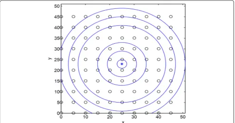
Considering that a WSN withNdistributed sensors and a target, we assume that noise exists among the target and the sensors. The noise is independent and identically distributed (i.i.d) and follows the standard Gaussian distri-bution with zero mean and unit variance. As Fig. 1 shows, Ndistributed sensors are uniformly deployed in the ROI which is a square with area A2, and a target randomly appears in the ROI. The locations of the local sensors are unknown to the FC, and every local sensor first monitors the ROI, makes a local decision about the target’s presence or absence, and then sends its decision to the FC to make a global decision which decides whether the target exists.
For a local sensori, the binary hypothesis testing problem is denoted as follows:
H1:ri¼siþni
H0:ri¼ni ð1Þ
where H1represents the hypothesis of the target’s pres-ence andH0represents the hypothesis of the target’s ab-sence. As discussed above, ni represents the noise and follows the standard Gaussian distribution
ni∼Nð0;1Þ ð2Þ
In Eq. (1), ri denotes the signal received by the local
sensor i, and si denotes the target’s signal detected by
the local sensori. The signal power emitted by the target decays as the distance from the target increases. The signal power attenuation model is as follows:
si¼g dð Þi ð3Þ
wheredi represents the distance between the target and the local sensoriis denoted as
di¼
and the function g(.) denotes the attenuation function with the distance from the target. In Eq. (4), (xi,yi)
rep-resents the coordinate of the local sensor i and (xt, yt)
represents the coordinate of the target. The functiong(.) has many different forms. One example for g(.) is de-noted in Eq. (21) as follows:
g xð Þ ¼ P0P0 x<d0 xβ x≥d0
ð5Þ
wherep0denotes the signal power emitted by the target at a reference distance d0, and β is the signal decay exponent. In Eq. (22), the functiong(.) which is used in this paper is given as follows:
g dð Þ ¼i
whereλis an adjustable constant andβoften takes values between 2 and 3. Assuming that the local sensoriuses the thresholdτito make the local binary decisionIi, in which
Idenotes that the target is present and 0 denotes that the target is absent, then all decisions denoted by I= (I1,I2, …,IN) are sent to the FC to make a global decision that 1 represents the target’s presence and 0 presents the target’s absence. According to the Neyman-Pearson (NP) lemma, the local sensor-level false alarm rate and probability of detection are given by
2dy, which is the
complemen-tary distribution function of the standard Gaussian. In WSNs for distribution detection, the local observa-tion has to be quantized before being transmitted to the FC which is demanded to make the final decision about the target’s presence.
3 Fusion rules
In this paper, we assume that all the local sensors have the same false alarm rate, that is, they have the same local threshold to make a local decision (Eqs. (21) and (22)). The local false alarm rate satisfies Eq. (7). We also assume that the wireless channels between the sensors and the fusion center are perfect, with negligible error rates. Three fusion rules will be shown in this section.
3.1K/Nfusion rule
K/N, which is short forKout ofN, is that the FC selects the data from the local sensors and makes a positive deci-sion when more thankdata values are“1”s. The formula of K/Nfusion rule is given by
Α1¼
where N is the total number of the sensors. When the FC receives the variable number of sensors, Eq. (9) can be written as
wheremdenotes that the total number of sensors which send data to the FC at the moment andk∈(0, 1),m≤N.
3.2 Counting rule
The counting rule, which is widely used as the fusion rule of the FC in Eqs. (6), (10), (22), and (23), is an intuitive choice that is to use the total number of“1”as a statistic. The counting rule makes a global decision by first count-ing the number of detections made by the local sensors and then comparing it with a thresholdT. The counting rule can be written as
Α3¼
PFa¼PrfΛ3≥TjH0g ð12Þ
wherePFais the global false alarm rate. When every local sensor has the same false alarm rate, the global false alarm rate can be written as
PFa¼X
When N is large enough, Eq. (13) can be obtained by using the Laplace-DeMoivre approximation
The threshold can be calculated as Eq. (22):
T¼Q−1ðPFaÞ
From Eq. (15), it is clear thatTis a function of the global false alarm rate, the local sensors’false alarm rate, and the total number of the sensors which send data to the FC.
3.3 LRFR
The LRFR uses the logistic regression to train the weights to make a decision. The logistic regression can be expressed as
h xð Þ ¼ 1
1þ exp −WTX ð16Þ
whereW is the weight vector, and xis the feature. xcan include the total number of the sensors which send data to the FC, the number of “1” reported by the sensors to the
FC, and the local sensors’performances (such as false alarm rate, detection probabilities), and the constant“1,”etc.
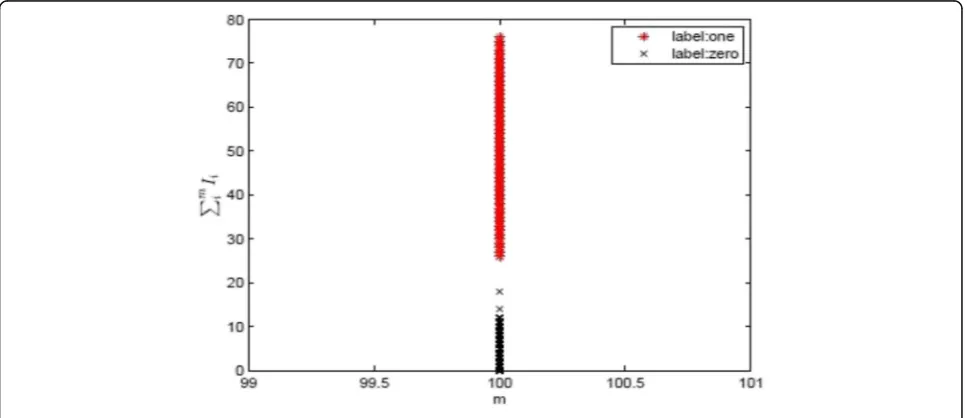
Ndenotes the total number of the sensors which send data to the FC. The equationm¼NXm
i¼1Ii denotes the
number of“1”reported by the local sensors. The red star means the target is present, and the black cross means the target is absent. A= 50,P0= 1500,τ= 1.6449,λ=
1,β= 2,N= 100.
As shown in Fig. 2, 10,000 simulations are conducted. The total number of the local sensors is 100 and fixed, that is, the FC selects data from the local sensors and makes a decision about the target’s presence when the data are equal to 100 at that moment. Some important parameters are set as follows: the area of ROI is 50, the power of the target is 1500, and the local sensors’ thresh-old is 1.6449. The red star denotes that the real circum-stance has the target. The black cross in Fig. 2 denotes that the real circumstance does not have the target. From Fig. 2, we can see that it has a clearly separable region between the target’s presence and the target’s absence.
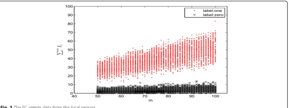
Ten thousand simulations are conducted in Fig. 3, where mis a variable that denotes the sensors’sent data to the FC at the moment. We assume that the FC makes a decision whenmis equal to or more than half of the initially total number of the local sensors at that moment. Some import-ant parameters are set as follows: the area of ROI is 50, the power of the target is 1500, and the local sensors threshold is 1.6449. The red star in Fig. 3 represents the target’s presence and the black cross represents the target’s absence. As shown in Fig. 3, it also has a clearly separable region between the target’s presence and the target’s absence.
So, whenNis known to the FC andm=N, the param-eters of the logistic regression can be set as follows:
w¼½w1 w0
x¼ Xm
i¼lIi 1
h i ð17Þ
wheremis a variable and more than or equal to half of
N. Xm
i¼1Ii denotes the number of “1” reported by the
local sensors. The red star means the target is present, and the black cross means the target is absent.A= 50,P0 = 1500,τ= 1.6449,λ= 1,β= 2,N= 100. Xm
i¼1Ii denotes
the number of“1”reported to the FC by the local sensors at that moment. Whenmis a variable, the parameters of the logistic regression can be obtained by
w¼½w1 w2 w0
x¼ mXm
i¼lIi 1
h i ð18Þ
The LRFR can be obtained by
where sign(x) is the sign function, h(x) stands for Eq. (16), and φ is a constant. The miss alarm rate rises with increasingφ, and the false alarm rate rises with decreasing
φ. Let φ= 0.5, we have WTx= 0. So, Eq. (19) can be simplified as
Λ5¼signð Þx0HH10 ð20Þ
3.4 LRFA
One of the LRFR’s most important steps is to obtain the parameters. To solve the problem, we can get the pa-rameters by the maximum likelihood estimator. Let
P uð ¼1jx;wÞ ¼h xð Þ ð21Þ
P uð ¼0jx;wÞ ¼1−h xð Þ ð22Þ
where u denotes the FC’s decision, x denotes the input
of the features, w is the weight of the LRFR, and h(x) represents Eq. (16). Because of the fact thatu can only be 1 or 0, the likelihood function can be expressed by
P uð jx;wÞ ¼h xð Þuð1−h xð ÞÞ1−u ð23Þ
With the independent training samples, the likelihood function can be written as
Lð Þ ¼w Pðu xj ;wÞ ¼ΠM
where M is the number of the training samples. It will be easier to maximize the log likelihood
lð Þ ¼w log L wf ð Þg
To solve the parameters of the LRFR, penalized logis-tic regression is often used in ML. The general formula is as follows:
where P(w) is the penalized function. To minimize Eq. (26), we can use the gradient descent. In Eq. (24), as an optimization problem, binary classification L2 penalized logistic regression minimizes the following cost function
min 1
The LRFA is shown as pseudo-code in Algorithm 1. Step 1 is only in numerical simulations, that is, the LRFR does not need the knowledge of the performances of local sensors. Steps 2 and 4 select Eq. (17) or Eq. (18) with the dependence of whether the total number of the sensors which send data to the FC is variable. Steps 3 and 4 train the LRFR with L1 and L2, respectively. The performances of the LRFR with L1 and L2 are computed, and a proper LRFR (step 4 in Algorithm 1) is selected. Through the LRFA, a proper LRFR is selected as the fusion rule of the FC.X
m
i¼1Ii denotes the number of “1” reported by the
local sensors, wherem=N. The red star means the tar-get is present, and the black cross means the tartar-get is absent.A= 50,P0= 1500,τ= 1.6449,λ= 1,β= 2,N= 100.
The mis a variable and more than or equal to half of N. Xm
i¼1Ii denotes the number of “1” reported by the
local sensors. The red star means the target is present, and the black cross means the target is absent. A= 50, P0= 1500,τ= 1.6449,λ= 1,β= 2,N= 100.
4 Numerical simulations
In this section, we conduct numerical simulations. The software of the numerical simulations used in this sec-tion are Matlab and Python. One of the packages of the Python is scikit-learn (Eq. (24)). Scikit-learn is on ML in Python, which is a simple and efficient tool for data mining and data analysis. It includes classification, regression, clustering, dimensionality reduction, model selection, and reprocessing.
As shown in Fig. 4, 1000 training samples are used to train the weights of Eq. (17). Some important parameters
are set as follows:A= 50,P0= 1500,τ= 1.6449,λ= 1,β=
2,N= 100. The number of the local sensors which send their data to the FC is fixed, that is, the FC makes a de-cision about the target’s presence when detections sent to the FC are up toN. We get the weights of Eq. (17) by the LRFA, and we generate 1000 random samples to test. From Fig. 4, the two labels of test samples can be clearly separated.
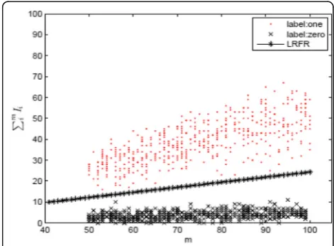
To show the influences of the variable total number of the local sensors which send data to the FC at that mo-ment, in Fig. 5, we assume that the FC makes decisions when the number of detections sent to the FC at that mo-ment is equal to or more than half of the initially total number of sensors deployed in ROI. The weights of Eq. (18) are trained by 1000 training samples. Some important parameters are set:A= 50,P0= 1500,τ= 1.6449,λ= 1,β=
2,N= 100. In this simulation, we can see the LRFR clearly separate the two labels (in Fig. 5).
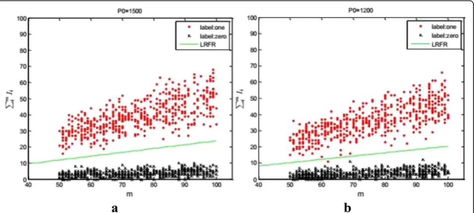
To see the influences of the different power of the target, we conduct variable powered experiments. The power of the target varies from 1500 to 100. The weights of Eq. (18) are solved by 10,000 training samples. Some important parameters are set: A= 50,τ= 1.6449,λ= 1,β= 2,N= 100, L=L2. From Fig. 6, the region between the two labels becomes small with the decrease of the target power. From
Eqs. (1) and (6), we know the received signal of the local sensors decreases with the decreasing power. The weights of Eq. (18) are solved by the 10,000 training samples. The LRFR can classify the target’s presence and absence with 1000 random test samples. Table 1 shows the performances of the FC change with the power of the target. The detected probability of the FC becomes small, and the false alarm rate of the FC becomes large with the power decreasing.
Figure 7 shows the comparison between LRFR andK/ N. Some important parameters are set:A= 50,P0= 1500,
τ= 1.6449,λ= 1, β= 2, N= 100. The LRFR can have the same ability of the k/N. However, there are no good
Fig. 6The variable total local sensors. Themis a variable and more than or equal to half ofN.Xm
i Iidenotes the number of“1”reported by the local sensor. Thered starmeans the target is present, and theblack crossmeans the target is absent.A= 50,τ= 1.6449,λ= 1,β= 2,N= 100.aP0= 1500. bP0= 900
Table 1The performances of the system with varying power
P0 1500 1200 900 600 300 100
PD 99.96% 99.96% 99.94% 99.80% 99.10% 94.72%
PFa 0% 0% 0% 0.18% 0.92% 9.60%
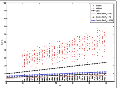
methods to solve the parameterkof theK/Nfusion rule. The LRFR can be easily solved by the ML method. To study the difference between the LRFR and the counting rule, in Fig. 8, the parameters are the same as Fig. 7. The performances of counting rule become decreasing with the global increasing false alarm rate. From Eq. (15), we know that the performances of the counting rule have the relation with the global false alarm rate.
5 Conclusions
In this paper, we give the general formula of thek/N fu-sion rule based on the total number of detections made by the local sensors. The LRFR and LRFA are proposed. The fixed total number of detections and the variable number of detections made by the local sensors are considered. The numerical simulations are given as above. From the numerical simulations, we see the LRFR can be well used as the FC’s fusion rule because of the outstanding performances and low computational com-plexity. One of the drawbacks of the LRFR is that it re-quires training samples to solve the weights of the LRFR. In the future, different methods of the ML will be
studied to solve the problems of the target detection and different features will be considered.
Authors’information
Longgeng Liu (b. June 5, 1975) received his M.Sc. in Computer Science (2000) from a university. Now, he is a director at China National Software and Integrated Circuit Promotion Center of the Ministry of Industry and Information Technology. He is a Ph.D. and studies at the University of Electronic Science and Technology. His current research interests include different aspects of artificial intelligence and distributed systems. He has (co-)authored more than two books and ten papers.
Competing interest
The authors declare that they have no competing interests.
Author details 1
University of Electronic Science and Technology, Chengdu, Sichuan 611731, China.2Chongqing University of Posts and Telecommunications, Chongqing 400065, China.
Received: 23 May 2016 Accepted: 12 December 2016
References
1. C. Fonseca, H. Ferreira, Stability and contagion measures for spatial extreme value analyses. arXiv. 1206-1228 (2012)
2. K Athanasios, Z Wang, A Rodrłguez, Spatial modeling for risk assessment of extreme values from environmental time series: a Bayesian nonparametric approach. Environmetrics23(8), 649–662 (2012)
3. N Katenka, E Levina, G Michailidis, Local vote decision fusion for target detection in wireless sensor networks. IEEE Trans. Signal. Process. ACM56(1), 329–338 (2008)
4. P. K. Varshney, Distributed detection and data fusion. New York: Springer-Verlag New York, Inc. 36-118 (1996)
5. I. Nevat, G. Peters, I. Collings, Distributed detection in sensor networks over fading channels with multiple antennas at the fusion center. 1(3), 45-49 (2014) 6. SH Javadi, A Peiravi, Fusion of weighted decisions in wireless sensor
networks. Wireless Sens. Syst. IET5(2), 97–105 (2015)
7. E Ermis, S Venkatesh, Distributed detection in sensor networks with limited range multimodal sensors. Signal. Process. IEEE Trans.58(2), 843–858 (2010) 8. Ridout, S Martin, An improved threshold approximation for local vote
decision fusion. Signal. Process. IEEE Trans.61(5), 1104–1106 (2013) 9. M Zhu et al., Fusion of threshold rules for target detection in wireless
sensor networks. ACM Trans. Sens. Netw. (TOSN)6(2), 18 (2010) 10. X Song et al., Active detection with a barrier sensor network using a scan
statistic. IEEE J. Ocean. Eng.37(1), 66–74 (2012)
11. M Guerriero, S Lennart, W Peter, Bayesian data fusion for distributed target detection in sensor networks. Signal. Process. IEEE Trans.58(6), 3417–3421 (2010) 12. M Guerriero, W Peter, G Joseph, Distributed target detection in sensor networks
using scan statistics. Signal. Process. IEEE Trans.57(7), 2629–2639 (2009) 13. J Glaz, Z Zhang, Multiple window discrete scan statistics. J. Appl. Stat.31(8),
967–980 (2004)
14. J Glaz, NI Naus, Tight bounds and approximations for scan statistic probabilities for discrete data. Ann. Appl. Probab.1(2), 306 (1991) 15. B Chen et al., Channel aware decision fusion in wireless sensor networks.
Signal. Process. IEEE Trans.52(12), 3454–3458 (2004)
16. R Hamid, V Azadeh, Optimal training and data power allocation in distributed detection with inhomogeneous sensors. Signal Processing Letters. IEEE.20(4), 339–342 (2013)
17. G Satish, R Niu, K Pramod, Fusing dependent decisions for hypothesis testing with heterogeneous sensors. Signal. Process. IEEE Trans.60(9), 4888–4897 (2012) 18. T Hastie et al.,The elements of statistical learning: data mining, inference, and
prediction. 2 (Springer, New York, 2009), pp. 65–104
19. C.M. Bishop, Pattern recognition and machine learning information science and statistics Secaucus. 2(3), 045-108 (2006)
Submit your manuscript to a
journal and benefi t from:
7Convenient online submission
7Rigorous peer review
7Immediate publication on acceptance
7Open access: articles freely available online
7High visibility within the fi eld
7Retaining the copyright to your article