Volume 2007, Article ID 65012,13pages doi:10.1155/2007/65012
Research Article
Mean Square Summability of Solution of Stochastic Difference
Second-Kind Volterra Equation with Small Nonlinearity
Beatrice Paternoster and Leonid Shaikhet
Received 25 December 2006; Accepted 8 May 2007
Recommended by Roderick Melnik
Stochastic difference second-kind Volterra equation with continuous time and small nonlinearity is considered. Via the general method of Lyapunov functionals construction, sufficient conditions for uniform mean square summability of solution of the considered equation are obtained.
Copyright © 2007 B. Paternoster and L. Shaikhet. This is an open access article distrib-uted under the Creative Commons Attribution License, which permits unrestricted use, distribution, and reproduction in any medium, provided the original work is properly cited.
1. Definitions and auxiliary results
Difference equations with continuous time are popular enough with researches [1–8]. Volterra equations are undoubtedly also very important for both theory and applications [3,8–12]. Sufficient conditions for mean square summability of solutions of linear sto-chastic difference second-kind Volterra equations were obtained by authors in [10] (for difference equations with discrete time) and [8] (for difference equations with continuous time). Here the conditions from [8,10] are generalized for nonlinear stochastic difference second-kind Volterra equations with continuous time. All results are obtained by general method of Lyapunov functionals construction proposed by Kolmanovski˘ı and Shaikhet [8,13–21].
Let{Ω,F,P}be a probability space and let{Ft, t≥t0}be a nondecreasing family of sub-σ-algebras ofF, that is,Ft1⊂Ft2fort1< t2, letHbe a space ofFt-adapted functions xwith valuesx(t) inRnfort≥t
0and the normx2=supt≥t0E|x(t)|2.
Consider the stochastic difference second-kind Volterra equation with continuous time:
xt+h0
=ηt+h0
+Ft,x(t),xt−h1
,xt−h2
and the initial condition for this equation:
x(θ)=φ(θ), θ∈Θ=
t0−h0−max j≥1 hj,t0
. (1.2)
Hereη∈H,h0,h1,. . .are positive constants,φis anFt0-adapted function forθ∈Θ, such
thatφ2
0=supθ∈ΘE|φ(θ)|2<∞, the functionalF with values inRnsatisfies the
condi-tion
F
t,x0,x1,x2,. . .2≤∞ j=0
ajxj 2
, A=∞
j=0
aj<∞. (1.3)
A solutionxof problem (1.1)-(1.2) is anFt-adapted processx(t)=x(t;t0,φ), which is equal to the initial functionφfrom (1.2) fort≤t0and with probability 1 defined by (1.1) fort > t0.
Definition 1.1. A functionxfromHis called
(i) uniformly mean square bounded ifx2<∞; (ii) asymptotically mean square trivial if
lim t→∞Ex(t)
2
=0; (1.4)
(iii) asymptotically mean square quasitrivial if for eacht≥t0,
lim j→∞Ex
t+jh02=0; (1.5)
(iv) uniformly mean square summable if
sup t≥t0
∞
j=0
Ext+jh0 2
<∞; (1.6)
(v) mean square integrable if
∞
t0
Ex(t)2dt <∞. (1.7)
Remark 1.2. It is easy to see that if the functionxis uniformly mean square summable, then it is uniformly mean square bounded and asymptotically mean square quasitrivial.
Together with (1.1), we will consider the auxiliary difference equation
xt+h0=Ft,x(t),xt−h1,xt−h2,. . .), t > t0−h0, (1.8)
with initial condition (1.2) and the functionalF, satisfying condition (1.3).
Definition 1.4. The trivial solution of (1.8) is called
(i) mean square stable if for any>0 andt0≥0, there exists aδ=δ(,t0)>0 such thatx(t)2<for allt≥t
0ifφ20< δ;
(ii) asymptotically mean square stable if it is mean square stable and for each initial functionφ, condition (1.4) holds;
(iii) asymptotically mean square quasistable if it is mean square stable and for each initial functionφand eacht∈[t0,t0+h0), condition (1.5) holds.
Below some auxiliary results are cited from [8].
Theorem1.5. Let the processηin (1.1) be uniformly mean square summable and there exist a nonnegative functionalV(t)=V(t,x(t),x(t−h1),x(t−h2),. . .), positive numbersc1,c2, and nonnegative functionγ: [t0,∞)→R, such that
γ= sup s∈[t0,t0+h0)
∞
j=0
γs+jh0
<∞, (1.9)
EV(t)≤c1sup s≤t
Ex(s)2, t∈t0,t0+h0
, (1.10)
EΔV(t)≤ −c2Ex(t) 2
+γ(t), t≥t0, (1.11)
whereΔV(t)=V(t+h0)−V(t). Then the solution of (1.1)-(1.2) is uniformly mean square summable.
Remark 1.6. Replace condition (1.9) inTheorem 1.5by condition
∞
t0
γ(t)dt <∞. (1.12)
Then the solution of (1.1) for each initial function (1.2) is mean square integrable.
Remark 1.7. If for (1.8) there exist a nonnegative functionalV(t)=V(t,x(t),x(t−h1),
x(t−h2),. . .), and positive numbersc1,c2such that conditions (1.10) and (1.11) (with
γ(t)≡0) hold, then the trivial solution of (1.8) is asymptotically mean square quasistable.
2. Nonlinear Volterra equation with small nonlinearity: conditions of mean square summability
Consider scalar nonlinear stochastic difference Volterra equation in the form
x(t+ 1)=η(t+ 1) + [t]+r
j=0
ajgx(t−j), t >−1,
x(s)=φ(s), s∈−(r+ 1), 0.
Herer≥0 is a given integer,aj are known constants, the processηis uniformly mean square summable, the functiong:R→Rsatisfies the condition
g(x)−x≤ν|x|, ν≥0. (2.2)
Below in Theorems 2.1, 2.7, new sufficient conditions for uniform mean square summability of solution of (2.1) are obtained. Similar results for linear equations of type (2.1) were obtained by authors in [8,10].
2.1. First summability condition. To get condition of mean square summability for (2.1), consider the matrices
with the solutionDthat is a symmetric matrix of dimensionk+ 1 with the elementsdi j. Put also
Theorem2.1. Suppose that for somek≥0, the solutionDof (2.4) is a positive semidefinite symmetric matrix such that the conditiondk+1,k+1>0holds. If besides of that
α2
then the solution of (2.1) is uniformly mean square summable.
Remark 2.2. Condition (2.6) can be represented also in the form
αk+1<
β2
k+dk−+1,1 k+1−βk. (2.8)
Remark 2.3. Suppose that in (2.1),aj=0 forj > k. Thenαk+1=0. So, if matrix equation (2.4) has a positive semidefinite solutionD withdk+1,k+1>0 andνis small enough to satisfy the inequality
ν< 1 α0
βk2+dk−+1,1 k+1−βk
, (2.9)
then the solution of (2.1) is uniformly mean square summable.
Remark 2.4. Suppose that the functiongin (2.1) satisfies the condition
g(x)−cx≤ν|x|, (2.10)
wherecis an arbitrary real number. Despite the fact that condition (2.10) is a more gen-eral one than (2.2), it can be used inTheorem 2.1 instead of (2.2). Really, if in (2.10)
c=0, then instead ofajandg in (2.1), one can useaj=ajcandg=c−1g. The function
gsatisfies condition (2.2) withν= |c−1|ν, that is,|g(x)−x| ≤ν|x|. In the casec=0, the proof ofTheorem 2.1can be corrected by evident way (seeAppendix A).
Remark 2.5. If inequalities (2.7), (2.8) hold and processη in (2.1) satisfies condition (1.12), then the solution of (2.1) is mean square integrable.
Remark 2.6. FromRemark 1.7, it follows that if inequalities (2.7), (2.8) hold, then the trivial solution of (2.1) withη(t)≡0 is asymptotically mean square quasistable.
2.2. Second summability condition. Put
α=∞ j=1
∞
m=0
am
, β= ∞
j=0
aj, (2.11)
A=α+1
2|β|, B=α
|β| −β, S=(1−β)(1 +β−2α)>0. (2.12)
Theorem2.7. Suppose that
β2+ 2α(1−β)<1, (2.13)
ν< 1
2|β|A
(A+B)2+ 2|β|AS−(A+B). (2.14)
Then the solution of (2.1) is uniformly mean square summable.
(For the proof ofTheorem 2.7, seeAppendix B.)
−3.5 −3 −2.5 −2 −1.5 −1 −0.5 0 0.5 1 1.5 2 2.5 3 3.5 a
−2.5
−2
−1.5
−1
−0.5 0.5 1 1.5 2 2.5
b
1 2
3
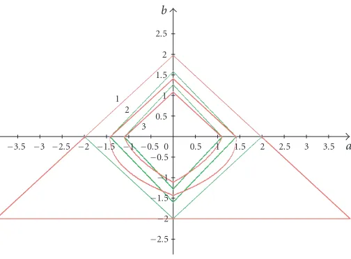
Figure 3.1. Regions of uniformly mean square summability for (3.1).
3. Examples
Example 3.1. Consider the difference equation
x(t+ 1)=η(t+ 1) +agx(t)+bgx(t−1), t >−1,
x(θ)=φ(θ), θ∈[−2, 0], (3.1)
with the functiongdefined as follows:g(x)=c1x+c2sinx,c1=0,c2=0. It is easy to see that the functiongsatisfies condition (2.10) withc=c1andν= |c2|. ViaRemark 2.4and (2.5), (2.6) for (3.1) in the casek=0, we haveα0= |c1|(|a|+|b|),α1= |c1b|,β0= |c1a|. Matrix equation (2.4) by the condition|c1a|<1 givesd11−1=1−c21a2>0.
So, conditions (2.7), (2.8) viaν= |c−1
1 c2|take the form
|a|+|b|<1 c1,
c2<c1c−2
1 − |ab| −(3/4)b2− |a| −(1/2)|b|
|a|+|b| . (3.2)
In the casek=1, we haveα0= |c1|(|a|+|b|),α1= |c1b|,α2=0. Besides (see [19]),
β1=c1
|b|+ |a| 1−c1b
, d−221=1−c21b2−c21a2 1 +c1b
1−c1b (3.3)
andd22is a positive one by the conditions|c1b|<1,|c1a|<1−c1b. Condition (2.8) trivially holds and condition (2.7) viaν= |c−1
1 c2|takes the form
c2<1−c1b1−c1a/1−c1b
|a|+|b| . (3.4)
c1=0.5 and different values ofc2: (1) c2=0, (2)c2=0.2, (3)c2=0.4. On the figure, one can see that forc2=0, condition (3.4) is better than (3.2) but for positivec2, both conditions add to each other. Note also that for negativec1, condition (3.4) gives a region that is symmetric about the axisa.
Example 3.2. Consider the difference equation
x(t+ 1)=η(t+ 1) +agx(t)+ In accordance withRemark 2.4, we will consider the parametersc1aandc1bjinstead ofaandbj. Via (2.11) by assumption|b|<1, we obtain
To obtain another condition for uniformly mean square summability of the solution of (3.5), transform the sum from (3.5) fort >0 in the following way:
[t]+r
Substituting (3.8) into (3.5), we transform (3.5) to the equivalent form
−2 −1.5 −1 −0.5 0 0.5 1 1.5 2 a
−2.5
−2
−1.5
−1
−0.5 0.5
b
1 2
3
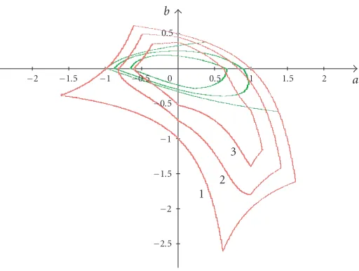
Figure 3.2. Regions of uniformly mean square summability given by conditions (3.7) and (3.10).
Using representation (3.9) of (3.5) without the assumption|b|<1, one can show (see Appendix C) that by conditions|c1b(1−a)|<1,|c1a+b|<1−c1b(1−a) and
c2<
1−c1b(1−a)1−c1a+b/1−c1b(1−a)
|a|+b(1−a) , (3.10)
the solution of (3.5) is uniformly mean square summable.
Regions of uniformly mean square summability given by conditions (3.7) (the green curves), (3.10) (the red curves) are shown onFigure 3.2forc1=1 and different values of
c2: (1)c2=0, (2)c2=0.2, (3)c2=0.6. On the figure, one can see that forc2=0, condition (3.10) is better than (3.7), but for other values ofc2, both conditions add to each other. For negativec1, condition (3.10) gives a region that is symmetric about the axisa.
Appendices
A. Proof ofTheorem 2.1
In the linear case (g(x)=x), this result is obtained in [19]. So, here we will stress only the features of nonlinear case.
[8,13–21] represents (2.1) in the form
We will construct the Lyapunov functionalV for (A.1) in the formV=V1+V2, where
V1(t)=X(t)DX(t),X(t)=(x(t−k),. . .,x(t−1),x(t)).
Then (A.3) takes the form
EΔV1(t)≤ −Ex2(t) +γ(t) +dk+1,k+1 [t]+r
m=0
Following GMLFC, choose the functionalV2as follows: Since the processη is uniformly mean square summable, then the functionγ satisfies condition (1.9). So if
q0dk+1,k+1<1, (A.9)
then the functionalV satisfies condition (1.11) ofTheorem 1.5. It is easy to check that condition (1.10) holds too. So if condition (A.9) holds, then the solution of (2.1) is uni-formly mean square summable.
then there exists a bigμ >0 so that condition (A.9) holds, and therefore the solution of (2.1) is uniformly mean square summable. It is easy to see that (A.11) is equivalent to conditions ofTheorem 2.1.
B. Proof ofTheorem 2.7
Represent now (2.1) as follows:
x(t+ 1)=η(t+ 1) +F1(t) +F2(t) +ΔF3(t), (B.1)
Following GMLFC, we will construct the Lyapunov functionalV for (2.1) in the form
V=V1+V2, whereV1(t)=(x(t)−F3(t))2. Calculating and estimatingEΔV1(t) via rep-resentation (B.1), similar to [8] we obtain
whereμ >0,αis defined by (2.11),λν=(1 +ν)(|β−1|+ν|β|+μ−1). ChoosingV2in the form
V2(t)=λν [t]+r
m=1
αmx2(t−m), αm=
∞
j=m
Bj, m=1, 2,. . ., (B.4)
for the functionalV=V1+V2, similar to [8] we have
EΔV(t)≤1 +μ(1 +ν)α+|β|Eη2(t+ 1) +β2−1 + 2α(1 +ν)|β−1|+ν|β|
+ν|β|+ν2β2+μ−1α(1 +ν)1 +|β|Ex2(t).
(B.5)
Thus, if
β2+ 2α(1 +ν)|β−1|+ν|β|+ν|β|+ν2β2<1, (B.6)
then there exists a bigμ >0 so that the functionalV satisfies the conditions ofTheorem 1.5, and therefore, the solution of (2.1) is uniformly mean square summable. It is easy to check that (B.6) is equivalent to conditions ofTheorem 2.7.
C. Proof of condition (3.10)
Following GMLFC, represent (3.9) in the form
x(t+ 1)=η(t+ 1) +F1(t) +F2(t), (C.1)
whereF1(t)=a0x(t) +a1x(t−1),F2(t)=a0g(x(t)) +a1g(x(t−1)),a0=a,a1=b(1−a),
a0=c1a+b,a1=c1a1,g(x)=g(x)−c1x. Using system (C.1) asX(t+ 1)=AX(t) +B(t), where
X(t)=
x(t−1)
x(t)
, A=
0 1
a1 a0
, B=
0
η(t+ 1) +F2(t)
, (C.2)
one has to repeat the proof ofTheorem 2.1. Equation (2.4) with the matrixA=Aby the conditions|a1|<1,|a0|<1−a1has a positive semidefinite solutionDsuch that
d−221=1−a21−a20 1 +a1
1−a1 >0. (C.3)
Since for (3.9)α2=0, then similar to (A.11) we obtainc22α20+ 2β1c2α0<d−221, where
α0=a0+a1= |a|+b(1−a), β1= a1+ a0
1−a1=
c1b(1−a)+c1a+b
c1b(1−a). (C.4)
References
[1] M. Gss. Blizorukov, “On the construction of solutions of linear difference systems with contin-uous time,”Differentsial’nye Uravneniya, vol. 32, no. 1, pp. 127–128, 1996, translation inDiff er-ential Equations, vol. 32, no. 1, pp. 133–134, 1996.
[2] D. G. Korenevski˘ı, “Criteria for the stability of systems of linear deterministic and stochastic difference equations with continuous time and with delay,”Matematicheskie Zametki, vol. 70, no. 2, pp. 213–229, 2001, translation inMathematical Notes, vol. 70, no. 2, pp. 192–205, 2001. [3] J. Luo and L. Shaikhet, “Stability in probability of nonlinear stochastic Volterra difference
equa-tions with continuous variable,”Stochastic Analysis and Applications, vol. 25, no. 3, 2007. [4] A. N. Sharkovsky and Yu. L. Ma˘ıstrenko, “Difference equations with continuous time as
math-ematical models of the structure emergences,” inDynamical Systems and Environmental Models (Eisenach, 1986), Math. Ecol., pp. 40–49, Akademie, Berlin, Germany, 1987.
[5] H. P´eics, “Representation of solutions of difference equations with continuous time,” in Pro-ceedings of the 6th Colloquium on the Qualitative Theory of Differential Equations (Szeged, 1999), vol. 21 ofProc. Colloq. Qual. Theory Differ. Equ., pp. 1–8, Electronic Journal of Qualitative The-ory of Differential Equations, Szeged, Hungary, 2000.
[6] G. P. Pelyukh, “Representation of solutions of difference equations with a continuous argument,” Differentsial’nye Uravneniya, vol. 32, no. 2, pp. 256–264, 1996, translation inDifferential Equa-tions, vol. 32, no. 2, pp. 260–268, 1996.
[7] Ch. G. Philos and I. K. Purnaras, “An asymptotic result for some delay difference equations with continuous variable,”Advances in Difference Equations, vol. 2004, no. 1, pp. 1–10, 2004. [8] L. Shaikhet, “Lyapunov functionals construction for stochastic difference second-kind Volterra
equations with continuous time,”Advances in Difference Equations, vol. 2004, no. 1, pp. 67–91, 2004.
[9] V. B. Kolmanovski˘ı, “On the stability of some discrete-time Volterra equations,”Journal of Ap-plied Mathematics and Mechanics, vol. 63, no. 4, pp. 537–543, 1999.
[10] B. Paternoster and L. Shaikhet, “Application of the general method of Lyapunov functionals construction for difference Volterra equations,”Computers & Mathematics with Applications, vol. 47, no. 8-9, pp. 1165–1176, 2004.
[11] L. Shaikhet and J. A. Roberts, “Reliability of difference analogues to preserve stability properties of stochastic Volterra integro-differential equations,”Advances in Difference Equations, vol. 2006, Article ID 73897, 22 pages, 2006.
[12] V. Volterra,Lesons sur la theorie mathematique de la lutte pour la vie, Gauthier-Villars, Paris, France, 1931.
[13] V. B. Kolmanovski˘ı and L. Shaikhet, “New results in stability theory for stochastic functional-differential equations (SFDEs) and their applications,” inProceedings of Dynamic Systems and Applications, Vol. 1 (Atlanta, GA, 1993), pp. 167–171, Dynamic, Atlanta, Ga, USA, 1994. [14] V. B. Kolmanovski˘ı and L. Shaikhet, “General method of Lyapunov functionals construction for
stability investigation of stochastic difference equations,” inDynamical Systems and Applications, vol. 4 ofWorld Sci. Ser. Appl. Anal., pp. 397–439, World Scientific, River Edge, NJ, USA, 1995. [15] V. B. Kolmanovski˘ı and L. Shaikhet, “A method for constructing Lyapunov functionals for
sto-chastic differential equations of neutral type,”Differentsial’nye Uravneniya, vol. 31, no. 11, pp. 1851–1857, 1941, 1995, translation inDifferential Equations, vol. 31, no. 11, pp. 1819–1825 (1996), 1995.
[16] V. B. Kolmanovski˘ı and L. Shaikhet, “Some peculiarities of the general method of Lyapunov functionals construction,”Applied Mathematics Letters, vol. 15, no. 3, pp. 355–360, 2002. [17] V. B. Kolmanovski˘ı and L. Shaikhet, “Construction of Lyapunov functionals for stochastic
[18] V. B. Kolmanovski˘ı and L. Shaikhet, “About one application of the general method of Lyapunov functionals construction,”International Journal of Robust and Nonlinear Control, vol. 13, no. 9, pp. 805–818, 2003, special issue on Time-delay systems.
[19] L. Shaikhet, “Stability in probability of nonlinear stochastic hereditary systems,”Dynamic Sys-tems and Applications, vol. 4, no. 2, pp. 199–204, 1995.
[20] L. Shaikhet, “Modern state and development perspectives of Lyapunov functionals method in the stability theory of stochastic hereditary systems,”Theory of Stochastic Processes, vol. 18, no. 1-2, pp. 248–259, 1996.
[21] L. Shaikhet, “Necessary and sufficient conditions of asymptotic mean square stability for sto-chastic linear difference equations,”Applied Mathematics Letters, vol. 10, no. 3, pp. 111–115, 1997.
Beatrice Paternoster: Dipartimento di Matematica e Informatica, Universita di Salerno, 84084 Fisciano (Sa), Italy
Email address:[email protected]
Leonid Shaikhet: Department of Higher Mathematics, Donetsk State University of Management, Chelyuskintsev 163-a, 83015 Donetsk, Ukraine