A delayed Holling type III functional response predator prey system with impulsive perturbation on the prey

R E S E A R C H

Open Access

A delayed Holling type III functional

response predator-prey system with

impulsive perturbation on the prey

Shunyi Li and Wenwu Liu

*_{Correspondence:}

A Holling type III functional response predator-prey system with constant gestation time delay and impulsive perturbation on the prey is investigated. The sufficient conditions for the global attractivity of a predator-extinction periodic solution are obtained by the theory of impulsive differential equations,i.e.the impulsive period is less than the critical valueT₁∗. The conditions for the permanence of the system are investigated,i.e.the impulsive period is larger than the critical valueT₂∗. Numerical examples show that the system has very complex dynamic behaviors, including (1) high-order periodic and quasi-periodic oscillations, (2) period-doubling and -halving bifurcations, and (3) chaos and attractor crises. Further, the importance of the impulsive period, the gestation time delay, and the impulsive perturbation

proportionality constant are discussed. Finally, the impulsive control strategy and the biological implications of the results are discussed.

Keywords: predator-prey system; impulsive perturbation; time delay; extinction; permanence; chaos

1 Introduction

The time delay population dynamics system describes the current state of the population not only related to the current state but also related to the state of the population in the past. That is to say, the time delay effect is very important in population dynamics, which tends to destabilize the positive equilibria and cause a loss of stability, bifurcate into var-ious periodic solutions, even make chaotic oscillations. Recently, there has been much work dealing with time delayed population systems (see [–]). For example, a stage-structured prey-predator system with time delay and Holling type-III functional response is considered by Wanget al.[], the existence and properties of the Hopf bifurcations are established. A delayed eco-epidemiology model with Holling-III functional response was instigated by Zouet al.[], and one found that time delay may lead to Hopf bifur-cation under certain conditions. The Hopf bifurbifur-cation of a delayed predator-prey system with Holling type-III functional response also has been considered in [–]. The exis-tence of positive periodic solutions of a delayed nonautonomous prey-predator system with Holling type-III functional response was considered in [–], by using the continu-ation theorem of coincidence degree theory. Therefore, time delays would make the

predator system subject to periodic oscillations via a local Hopf bifurcation, and destroy the stability of the system.

Recently, more and more authors have discussed the impulsive perturbation on prey-predator systems, since the system would be stabilized by impulsive effects, and would make the system subject to complex dynamical behaviors [–]. For example, a predator-prey model with impulsive effect and generalized Holling type III functional response was studied by Suet al.[], and the sufficient conditions for the existence of a pest-eradication periodic solution and permanence of the system are obtained. The existence of positive periodic solutions of the nonautonomous prey-predator system with Holling type III func-tional response and impulsive perturbation is considered in [, ]. By using a continua-tion theorem of coincidence degree theory, the sufficient condicontinua-tions for the existence of a positive periodic solution are obtained for the system.

Note that harmful delays would destroy the stability of the system via bifurcations and even lead the system to extinction. At this point, the impulsive control strategies can be considered, which can both improve the stability of the system and control the amplitude of the bifurcated periodic solution effectively. For example, a time delayed Holling type II functional response prey-predator system with impulsive perturbations is investigated by Jiaet al.[], and the problems of the predator-extinction periodic solution and the permanence of the system are investigated. So, how does the dynamical behavior go when the delayed system with impulsive effect? Especially, what would happen for the delayed predator-prey system with Holling type III functional response under impulsive pertur-bation?

Motivated by the aforementioned observations, we assume the predator needs a certain time to gestate the prey, and we consider the following delayed Holling type III functional response prey-predator system with impulsive perturbation on the prey:

⎧

β,k,dare positive.ris the intrinsic rate of increase of the prey,Kis the carrying capacity of the prey.α is the predation coefficient of the predator, which reflects the size of the predator’s ability, andβ is predation regulation factor (saturation factor) of the predator.

dis the death rate of the predator,k( <k< ) is the rate of conversing prey into predator.

x(t) =x(t+) –x(t),y(t) =y(t+) –y(t),Tis the impulsive periodic.n∈N+,N+={, , . . .},

p>  is the proportionality constant which represents the rate of mortality due to the applied pesticide. The initial conditions for system () are

examples are given to support the theoretical research, and some complex dynamic be-haviors are shown. For example, we see period-halving and period-doubling bifurcations, periodic and high-order quasi-periodic oscillations, even chaotic oscillation. The impor-tance of the impulsive periodT, the gestation time delayτ, and the impulsive perturbation proportionality constantpare discussed. Finally, the impulsive control strategy and bio-logical implications of the results are discussed.

2 Preliminaries

LetR+= [,∞),R+={x∈R|x≥}. Denote byf = (f,f) the map defined by the right

hand of the first two equations of system (), and letNbe the set of all non-negative inte-gers. LetV:R+×R+→R+, thenVis said to belong to classVif:

() Vis continuous in(t,x)∈(nT, (n+ )T]×R

+and for eachx∈R+,n∈N, lim(t,y)→(nT+_,x)V(t,y) =V(nT+,x)exists.

() Vis locally Lipschitzian inx.

Definition . LetV∈V, then for (t,x)∈(nT, (n+ )T]×R+, the upper right derivative

ofV(t,x) with respect to the impulsive differential system () is defined as

D+V(t,x) = lim

Definition . System () is said to be permanent if there exist two positive constants

m,M, andTsuch that each positive solutionX(t) = (x(t),y(t)) of the system () satisfies

m≤x(t)≤M,m≤y(t)≤Mfor allt>T.

The solution of system () is a piecewise continuous functionx:R+→R+,x(t) is

contin-uous on (nT, (n+ )T],n∈N, andx(nT+_{) =lim}

t→nT+x(t) exists, the smoothness properties

off guarantee the global existence and uniqueness of solutions of system (), for details see [, ].

solution of the scalar impulsive differential equation

We consider the following subsystem of system ():

is a globally asymptotically stable positive periodic solution of system () [].

Lemma . If( –p)erT _{> ,system()has a predator-extinction periodic solution X(t) =} (x∗(t), )for t∈(nT, (n+ )T],and for any solution X(t) = (x(t),y(t))of system(),we have x(t)→x∗(t)as t→+∞.

Lemma . Consider the following delay differential equation[]:

x(t) =ax(t–τ) –bx(t), second equation of system (), we get

y(t)≤kα

β y(t–τ) –dy(t).

Consider the following delayed comparison equation:

increasing function about variablez. Therefore, there exists a sufficiently small positive constantεsuch that

kα(X∗_+ε)

 +β(X_∗+ε) –d< .

By the first and third equations of system (), we have

x(t)≤rx(t)( –x_K(t)), t=nT,

x(t) = –px(t), t=nT,

then we consider the following comparison system:

z(t) =rz(t)( –z_K(t)), t=nT,

z(t) = –pz(t), t=nT, ()

withz(+) =z() =x(). Recalling system (), we obtain a unique globally asymptotically stable positiveT-periodic solution of system (), where

z∗(t) = K

[_(–e_prT_)e–rT_–– ]e–r(t–nT)+ 

, t∈nT, (n+ )T.

Then, there exists an arbitrarily small positive constantεandn∈Nsuch that

x(t)≤z∗(t) +ε≤ K

fort≥nT+τ. Consider the following delayed comparison equation:

with initial conditionz(+) =x(+). From (), we get

By the first equation of system (), we get

x(t)≤rx(t)

right derivative ofV(t) along a solution of system ():

Consider the following differential inequalities:

V(t)≤–dV(t) +M, t=nT,

V(t+)≤V(t), t=nT, according to Lemma ., we have

V(t)≤

positive solution of system () is uniformly ultimately bounded.

Denote conditions (). Rewrite the second equation of system () as follows:

dy(t)

CalculatingV(t) along the solution of system (), we have

V(t) =d

Since> , there exist two positive constantsm∗andεsmall enough such that

By the first and third equations of system (), we obtain

exists a nonnegative constantTsuch that

y(t)≥y (T≤t≤T+T+τ), y(T+T+τ) =y, y(T+T+τ)≤.

Thus, by the second equation of system (), (), and (), we obtain

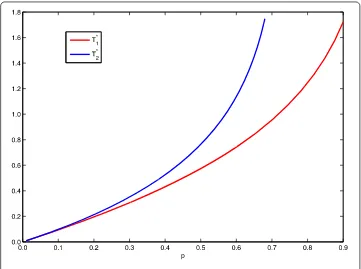
Figure 1 The two thresholdsT₁∗andT∗₂for system (18).

On the one hand, if y(t)≥m∗_ holds true for all sufficiently larget, then our aim is reached. On the other hand, supposey(t) is oscillatory aboutm∗_. Let m=min{m∗/,

m∗_exp(–dτ)}and we will prove thaty(t)≥m. There exist two positive constants¯tandω

such thaty(¯t) =y(t¯+ω) =m∗_andy(t) <m∗_fort∈(¯t,t¯+ω). The inequalityx(t) >ρholds true fort∈(¯t,t¯+ω) when¯tis large enough.

Since there is no impulsive effect ony(t),y(t) is uniformly continuous. Then, there exists a constantT(with  <T<τandTis dependent of the choice of¯t) such thaty(t) >m∗/

for allt∈[¯t,t¯+T].

Ifω≤T, our aim is reached. IfT<ω≤τ, by the second equation of system () we get

y(t)≥–dy(t) fort∈(t¯,¯t+ω]. Then we gety(t)≥m∗_exp(–dτ) fort¯<t≤ ¯t+ω≤ ¯t+τsince

y(t) =m∗_. Therefore,y(t)≥mfort∈(¯t,¯t+ω].

Ifω≥τ, from the second equation of system (), then we gety(t)≥mfort∈(¯t,¯t+τ].

Thus, we havey(t)≥m fort∈[¯t+τ,¯t+ω]. According to the above proof. Since the

interval [¯t,t¯+ω] is arbitrarily chosen, we havey(t)≥mfor sufficiently larget. From our

arguments above, the choice ofm is independent of the positive solution of system ()

which shows thaty(t)≥mholds for sufficiently larget.

By Theorem ., we obtainy(t)≤Yfor sufficiently larget. Therefore, by the first

equa-tion of system (), we get

x(t)≥rx(t)

 –x(t)

K

for sufficiently larget, wherer=r–αKY andK=K r/r. Therefore, we have x(t)≥

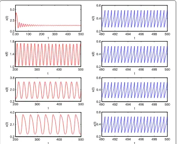
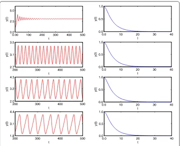
Figure 2 Time-series of prey populationx(t) of system (18) without (left) and with (right) impulsive periodT= 0.5 <T₁∗when the time delayτ= 0.5, 0.7, 3, 6, respectively.

the following comparison system:

z_(t) =rz(t)( –z_K(_t)), t=nT,

z(t) = –pz(t), t=nT,

with initial conditionz(+) =x(+). Similarly, we can choose aε>  small enough such

that

x(t) >z∗_(t) –ε≥K[( –p)e

rT_{– ]}

erT_{– } –εm

holds for sufficiently larget.

Remark  Let ( –p)erT _{>  and}

F

f(p,T)

= kαf

 (p,T)

d( +f_(p,T))– , f(p,T) =

K[( –p)erT– ] ( –p)(erT_{– )} .

Note thatF(f(p,T)) is a monotonically increasing function with respect tof(p,T), and

f(p,T) is a monotonically increasing function with respect toT(T> –ln( –p)/r) and a

monotonically decreasing function with respect top( <p<  –exp(–rT)), since

f_p(p,T) = –K

(erT_{– )( –p)} < , f

T(p,T) =

rpK erT

Figure 3 Time-series of predator populationy(t) of system (18) without (left) and with (right) impulsive periodT= 0.5 <T₁∗when time delayτ= 0.5, 0.7, 3, 6, respectively.

So, there exists a uniqueT_∗such thatF(f(p,T∗)) =  if we fixp, similarly, there exists a

uniquep∗_ such thatF(f(p∗,T)) =  if we fixT. Therefore, the condition<  is

equiva-lent toT<T_∗(orp>p∗_), whereT_∗(p∗_) is the unique solution ofF(f(p,T)) = .

Similarly, let

F

f(p,T)

= kαf

 (p,T)

d( +f (p,T))

– , f(p,T) =

K[( –p)erT_{– ]}

erT_{– } .

Note thatF(f(p,T)) is a monotonically increasing function with respect tof(p,T), and

f(p,T) is a monotonically increasing function with respect toT (T> –ln( –p)/r) and a

monotonically decreasing function with respect top( <p<  –exp(–rT)), since

f_p(p,T) = –K erT< , f_T(p,T) = rpK e rT

(erT_{– )}> .

So, there exists a uniqueT_∗such thatF(f(p,T∗)) =  if we fixp, similarly, there exists a

uniquep∗_such thatF(f(p∗,T)) =  if we fixT. Therefore, the condition>  is

equiv-alent toT>T_∗(orp<p∗_), whereT_∗(p∗_) is the unique solution ofF(f(p,T)) = .

Remark  Note thatf(p,T) >f(p,T), soT∗<T∗forF(f(p,T∗)) =  andF(f(p,T∗)) = 

Figure 4 Time-series of prey (left) and predator (right) populationy(t) of system (18) with impulsive periodT= 0.8 >T₂∗when the time delayτ= 0.5, 0.7, 3, 6, respectively.

a thresholdTmax. IfT<Tmax, then the prey- (or predator)-eradication periodic solution is

locally asymptotically stable; ifT>Tmaxthe system is permanent. But we get two

thresh-oldsT_∗andT_∗, and there is no information as regards the system whenT_∗<T<T_∗. This is essentially different when system () is with or without time delay.

4 Numerical analysis

Numerical experiments are carried out to integrate the system by using the DDE algo-rithm method in MATLAB.

4.1 Example 1

We consider the following delayed Holling type-III response prey-predator system with impulsive perturbation:

⎧ ⎪ ⎪ ⎪ ⎪ ⎪ ⎨ ⎪ ⎪ ⎪ ⎪ ⎪ ⎩

x(t) = .x(t)( –x(_t)) –._+x_x(t_(t)y₎(t),

y(t) = _[+x(t–_xτ)₍y_t–(t_τ–_)]τ)– .y(t),

t=nT,

x(t) = –px(t),

y(t) = , t=nT,

()

wherer= .,K= ,α= .,β= ,k= .,d= ., with initial conditions (φ(t),φ(t)) =

(, ),t∈[–τ, ]. From Remark , we can get thresholdsT_∗andT_∗when varying the values of parameterpfrom . to .. From Figure , we see thatT_∗gets more and more close toT∗whenpgets more and more close to zero.

According to [, ], there would be a time delay critical valueτ, and there is a Hopf

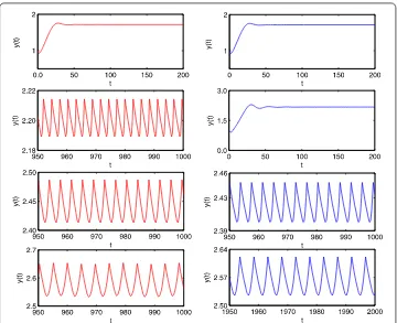
Figure 5 Time-series of prey (left) and predator (right) populationy(t) of system (18) with time delay

τ= 0.5 when the impulsive periodT= 1.8, 2.8, 3.8, 4.8, respectively.

impulsive perturbation (i.e. p= ). From the time-series of the prey population (Figure  (left)) and the predator population (Figure  (left)) with time delayτ= ., ., , , respec-tively, we know that the time delay critical valueτis between . and .. The prey and

predator populations are locally stable when the time delayτ≤. and coexist with sable cycles whenτ≥..

From Theorem ., Theorem ., and Remark , one knows that ifT<T_∗the predator-extinction periodic solution is globally attractive and ifT>T_∗the system has permanence. From Figure , we seeT_∗≈. andT_∗≈. whenp= .. Then, the predator-extinction periodic solution is globally attractive whenT= . <T∗(see Figure  (right)

and Figure  (right)) where the time delayτ = ., ., , , respectively. The system is permanent whenT= . >T_∗where the time delayτ= ., ., , , respectively (see Fig-ure ). Furthermore, when the time delayτ= . <τthe predator and prey populations

coexist with sable cycles, where the impulsive periodT= ., ., ., ., respectively (see Figure ). That is to say, an impulsive effect would destabilize the system under some con-ditions. If we increasing the time delay from  to ., that large time delay could stabilize the system (see Figure  and Figure ).

4.2 Example 2

Figure 6 Time-series of prey-predator populationy(t) of system (18) with time delayτ= 2 (left) and

τ= 2.5 (right) when the impulsive periodT= 1.8, 2.8, 3.8, 4.8, respectively.

⎧ ⎪ ⎪ ⎪ ⎪ ⎪ ⎨ ⎪ ⎪ ⎪ ⎪ ⎪ ⎩

x(t) = .x(t)( –x(_t)) – ._+.x(_xt)y_(t(₎t),

y(t) =._+.x(t_x–τ_(t)_–y_τ(t₎–τ)– .y(t),

t=nT,

x(t) = –px(t),

y(t) = , t=nT,

()

where r= .,K= , α= .,β= .,k= .,d= ., with initial condition (φ(s),

φ(s)) = (, ),s∈[–τ, ]. First of all, we letp= .,τ= , and we consider the effect of the

impulsive periodT on system (). The bifurcation diagrams of the impulsive periodT

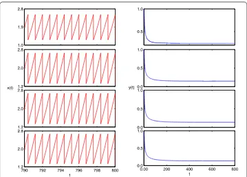
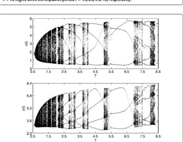
over [., .] and [., .], show that system () has complex dynamics (see Figure  and Figure ), including high-order periodic and quasi-periodic oscillating, period-doubling and period-halving bifurcations, and chaos and attractor crises. For example, there exist T, T, T periodic solutions whenT= ., ., ., respectively (see Figure ). When

T increases from . to ., there is an attractor crisis leading to a chaotic solution (see Figure ). These results imply that an impulsive effect could destroy the stability of the system and lead to multiple attractors, bifurcations, even chaos oscillations, which makes the dynamical behaviors very complex.

Figure 7 Time-series of prey predator populationy(t) of system (18) with time delayτ= 4 (left) and

τ= 4.8 (right) when the impulsive periodT= 1.8, 2.8, 3.8, 4.8, respectively.

Figure 9 Bifurcation diagrams of system (19): prey populationx(t) (top) and predator populationy(t) (bottom) whenp= 0.3,τ= 3 with impulsive periodTover [6.9, 7.5].

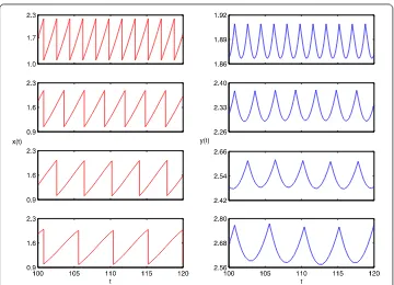
Figure 10 Phase portrait of the system (19).5T, 4T, 3Tperiodic solution whenT= 3.5, 4.5, 6.5, respectively.

Finally, we letτ= ,T= , and we investigate the impulsive perturbation proportion-ality constantpon system (). The bifurcation diagrams of impulsive perturbation pro-portionality constantpover [., .] show that system () has complex dynamics (see Figure ). These results imply that the impulsive perturbation proportionality constantp

Figure 11 Crisis are shown: from left to right there is a crisis that the chaos suddenly appears when T= 6.93, 6.94, respectively.

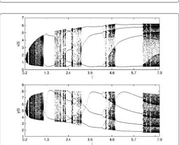
Figure 12 Bifurcation diagrams of system (19): prey populationx(t) (top) and predator population y(t) (bottom) whenp= 0.3,T= 7 with time delayτover [0.2, 7.0].

5 Conclusion

In this paper, we have investigated a prey-predator system with constant gestation time delay and impulsive perturbation on the prey in detail. We have shown that there exists a globally attractive predator-extinction periodic solution when the impulsive periodTis less than the critical valueT_∗. The system is permanent when the impulsive periodT is larger than the critical valueT_∗. Therefore, we get two thresholdsT_∗andT_∗, and there is no information as regards the system () whenT_∗<T<T_∗. If the system () is without time delay, thenT_∗=Tmax=T∗would be the unique threshold. This is essentially different

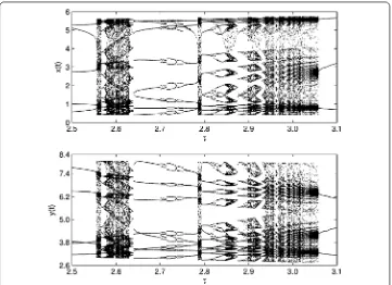
Figure 13 Bifurcation diagrams of system (19): prey populationx(t) (top) and predator population y(t) (bottom) whenp= 0.3,T= 7 with time delayτover [2.5, 3.1].

Figure 14 Period-doubling bifurcation leads to chaos. From left to right: phase portrait ofT-periodic, 2T-periodic solutions and chaos whenτ= 4.1, 4.2, 4.3, respectively.

Figure 15 Bifurcation diagrams of system (19): prey populationx(t) (top) and predator population y(t) (bottom) whenτ= 7,T= 7 with parameterpover [0.2, 0.74].

Competing interests

The authors declare that they have no competing interests.

Authors’ contributions

SL carried out the main part of this manuscript. WL participated in the discussion and gave the examples. All authors read and approved the final manuscript.

Acknowledgements

This work was supported by the Joint Natural Science Foundation of Guizhou Province (Nos. LKQS[2013]12 and LH[2014]7437); Foundation of Qiannan Normal College for Nationalities (Nos. 2014ZCSX03 and 2014ZCSX11).

Received: 19 October 2015 Accepted: 21 January 2016

References

1. Li, S, Xue, Y, Liu, W: Hopf bifurcation and global periodic solutions for a three-stage-structured prey-predator system with delays. Int. J. Inf. Syst. Sci.8(1), 142-156 (2012)

2. Li, S, Liu, W, Xue, X: Bifurcation analysis of a stage-structured prey-predator system with discrete and continuous delays. Appl. Math.4(7), 1059-1064 (2013)

3. Li, S, Xiong, Z: Bifurcation analysis of a predator-prey system with sex-structure and sexual favoritism. Adv. Differ. Equ.

2013, Article ID 219 (2013)

4. Wang, L, Xu, R, Feng, G: A stage-structured predator-prey system with time delay and Holling type-III functional response. Int. J. Pure Appl. Math.48(2), 53-66 (2008)

5. Zou, W, Xie, J, Xiong, Z: Stability and Hopf bifurcation for an eco-epidemiology model with Holling-III functional response and delays. Int. J. Biomath.1(3), 377-389 (2008)

6. Zhang, X, Xu, R, Gan, Q: Periodic solution in a delayed predator prey model with Holling type III functional response and harvesting term. World J. Model. Simul.7(1), 70-80 (2011)

7. Das, U, Kar, TK: Bifurcation analysis of a delayed predator-prey model with Holling type III functional response and predator harvesting. J. Nonlinear Dyn.2014, Article ID 543041 (2014)

8. Zhang, Z, Yang, H, Fu, M: Hopf bifurcation in a predator-prey system with Holling type III functional response and time delays. J. Appl. Math. Comput.44(1-2), 337-356 (2014)

9. Fan, Y, Wang, L: Multiplicity of periodic solutions for a delayed ratio-dependent predator-prey model with Holling type III functional response and harvesting terms. J. Math. Anal. Appl.365(2), 525-540 (2010)

10. Cai, Z, Huang, L, Chen, H: Positive periodic solution for a multi species competition-predator system with Holling III functional response and time delays. Appl. Math. Comput.217(10), 4866-4878 (2011)

12. Xu, C, Wu, Y, Lu, L: Permanence and global attractivity in a discrete Lotka-Volterra predator-prey model with delays. Adv. Differ. Equ.2014, Article ID 208 (2014)

13. Li, S: Complex dynamical behaviors in a predator-prey system with generalized group defense and impulsive control strategy. Discrete Dyn. Nat. Soc.2013, Article ID 358930 (2013)

14. Li, S, Xiong, Z, Wang, X: The study of a predator-prey system with group defense and impulsive control strategy. Appl. Math. Model.34(9), 2546-2561 (2010)

15. Su, H, Dai, B, Chen, Y, et al.: Dynamic complexities of a predator-prey model with generalized Holling type III functional response and impulsive effects. Comput. Math. Appl.56(7), 1715-1725 (2008)

16. Fan, X, Jiang, F, Zhang, H: Dynamics of multi-species competition-predator system with impulsive perturbations and Holling type III functional responses. Nonlinear Anal., Theory Methods Appl.74(10), 3363-3378 (2011)

17. Liu, Z, Zhong, S: An impulsive periodic predator-prey system with Holling type III functional response and diffusion. Appl. Math. Model.36(12), 5976-5990 (2012)

18. Yan, C, Dong, L, Liu, M: The dynamical behaviors of a nonautonomous Holling III predator-prey system with impulses. J. Appl. Math. Comput.47(1), 193-209 (2015)

19. Tan, R, Liu, W, Wang, Q: Uniformly asymptotic stability of almost periodic solutions for a competitive system with impulsive perturbations. Adv. Differ. Equ.2014, Article ID 2 (2014)

20. Xu, L, Wu, W: Dynamics of a nonautonomous Lotka-Volterra predator-prey dispersal system with impulsive effects. Adv. Differ. Equ.2014, Article ID 264 (2014)

21. Ju, Z, Shao, Y, Kong, W: An impulsive prey-predator system with stagestructure and Holling II functional response. Adv. Differ. Equ.2014, Article ID 280 (2014)

22. Jia, J, Cao, H: Dynamic complexities of Holling type II functional response predator-prey system with digest delay and impulsive. Int. J. Biomath.2(2), 229-242 (2009)

23. Bainov, DD, Simeonov, DD: Impulsive Differential Equations: Periodic Solutions and Applications. Longman, Harlow (1993)

24. Lakshmikantham, V, Bainov, DD, Simeonov, PS: Theory of Impulsive Differential Equations. World Scientific, Singapore (1989)