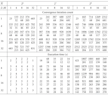
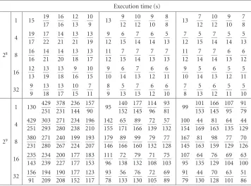
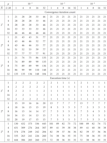
Monotone finite difference domain decomposition algorithms and applications to nonlinear singularly perturbed reaction diffusion problems

MONOTONE FINITE DIFFERENCE DOMAIN

DECOMPOSITION ALGORITHMS AND

APPLICATIONS TO NONLINEAR SINGULARLY

PERTURBED REACTION-DIFFUSION PROBLEMS

Received 16 September 2004; Revised 21 December 2004; Accepted 11 January 2005

This paper deals with monotone finite difference iterative algorithms for solving non-linear singularly perturbed reaction-diffusion problems of elliptic and parabolic types. Monotone domain decomposition algorithms based on a Schwarz alternating method and on box-domain decomposition are constructed. These monotone algorithms solve only linear discrete systems at each iterative step and converge monotonically to the ex-act solution of the nonlinear discrete problems. The rate of convergence of the mono-tone domain decomposition algorithms are estimated. Numerical experiments are pre-sented.

Copyright © 2006 Hindawi Publishing Corporation. All rights reserved.

1. Introduction

We are interested in monotone discrete Schwarz alternating algorithms for solving non-linear singularly perturbed reaction-diffusion problems.

The first problem considered corresponds to the singularly perturbed reaction-diff u-sion problem of elliptic type

−μ2_{uxx+uyy+f(x,y,u)=0, (x,y)∈ω,} u=g on∂ω, ω=ωx_×ωy_{= {0< x <1} × {0< y <1},}

fu≥c∗, (x,y,u)∈ω×(−∞,∞), fu≡∂ f /∂u,

(1.1)

whereμis a small positive parameter,c∗>0 is a constant,∂ω is the boundary ofω. If f andgare sufficiently smooth, then under suitable continuity and compatibility condi-tions on the data, a unique solutionuof (1.1) exists (see [6] for details). Furthermore, forμ1, problem (1.1) is singularly perturbed and characterized by boundary layers (i.e., regions with rapid change of the solution) of widthO(μ|lnμ|) near∂ω(see [1] for details).

Hindawi Publishing Corporation Advances in Difference Equations Volume 2006, Article ID 70325, Pages1–38

The second problem considered corresponds to the singularly perturbed reaction-diffusion problem of parabolic type

−μ2_{uxx+uyy+f(x,y,t,u) +ut=0, (x,y)∈ω,t∈(0,T],}

fu≥0, (x,y,t,u)∈ω×[0,T]×(−∞,∞), (1.2)

where ω= {0< x <1} × {0< y <1} and μis a small positive parameter. The initial-boundary conditions are defined by

u(x,y, 0)=u0(x,y), (x,y)∈ω,

u(x,y,t)=g(x,y,t), (x,y,t)∈∂ω×(0,T]. (1.3)

The functions f,g, andu0_{are sufficiently smooth. Under suitable continuity and} com-patibility conditions on the data, a unique solutionuof (1.2) exists (see [5] for details). Forμ1, problem (1.2) is singularly perturbed and characterized by the boundary lay-ers of widthO(μ|lnμ|) at the boundary∂ω (see [2] for details). We mention that the assumption fu≥0 in (1.2) can always be obtained via a change of variables.

In solving such nonlinear singularly perturbed problems by the finite difference method, the corresponding discrete problem is usually formulated as a system of non-linear algebraic equations. One then requires a reliable and efficient computational algo-rithm for computing the solution. A fruitful method for the treatment of these nonlinear systems is the method of upper and lower solutions and its associated monotone itera-tions (in the case of unperturbed problems with reaction-diffusion equations see [8,9] and the references therein). Since the initial iteration in the monotone iterative method is either an upper or lower solution constructed directly from the difference equations without any knowledge of the exact solution (see [3,4] for details), this method elimi-nates the search for the initial iteration as is often needed in Newton’s method. This gives a practical advantage in the computation of numerical solutions.

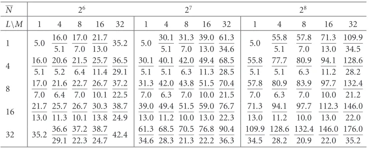
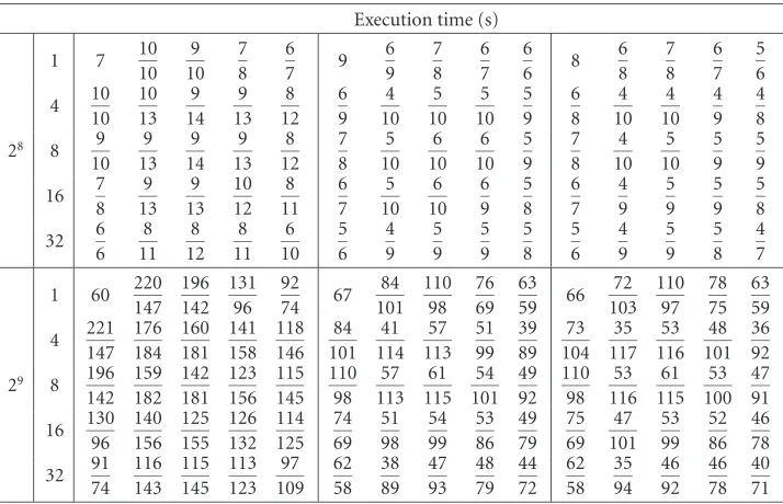
InSection 2, we introduce the classical nonlinear finite difference schemes for the nu-merical solution of (1.1) and (1.2). Iterative methods by which each of these schemes may be solved are presented in [3,4]. From an arbitrary initial mesh function, one may construct a sequence of functions which converges monotonically to the exact solution of the nonlinear difference scheme. Each function in the sequence is generated as the so-lution of a linear difference problem. InSection 3, we consider the elliptic problem and extend the monotone method to a box-decomposition of the computational domain. We show that monotonic convergence is maintained under the proposed decomposition and associated algorithm. Further, we develop estimates of the rate of convergence. The box-decomposition of the spatial domain is applied to the parabolic nonlinear difference scheme inSection 4. Numerical experiments are presented inSection 5. These confirm the theoretical estimates of the earlier sections. Suggestions are made regarding future parallel implementation.

2. Difference schemes for solving (1.1) and (1.2)

Onωand [0,T] introduce nonuniform meshesωh=ωhx_×ωhy_andωτ_:

ωhx_{=xi, 0≤i≤Nx;x}

0=0,xNx=1;hxi=xi+1−xi

, ωhy_{=yj, 0≤j≤Ny; y}

0=0, yNy=1; hy j=yj+1−yj

, ωτ_{=tk=kτ, 0≤k≤Nτ,Nττ=T.}

(2.1)

For approximation of the elliptic problem (1.1), we use the classical difference scheme on nonuniform meshes

ᏸh_{U+f(P,U)=0, P∈ω}h_,U=gon∂ωh_{, (2.2)}

whereᏸhUis defined by

ᏸh_{U= −μ}2_Ᏸ2

x+Ᏸ2yU, (2.3)

andᏰ2

xU(P),Ᏸ2yU(P) are the central difference approximations to the second derivatives

Ᏸ2

xUij=xi−1Ui+1,j−Uijhxi−1−Uij−Ui−1,jhx,i−1 −1

, Ᏸ2

yUij=y j−1Ui,j+1−Uijhy j−1−Uij−Ui,j−1hy,j−1−1

,

xi=2−1hx,i−1+hxi, y j=2−1hy,j−1+hy j,

(2.4)

To approximate the parabolic problem (1.2), we use the implicit difference scheme ᏸhτ_{U(P,t) + f(P,t,U)=τ}−1_{U(P,t−τ), (P,t)∈ω}h_×ωτ_,

ᏸhτ_U(P,t)≡ᏸh_{U(P,t) +τ}−1_U(P,t),

U(P, 0)=u0_{(P), P∈ω}h_{, U(P,t)=g(P,t), (P,t)∈∂ω}h_×ωτ_,

(2.5)

whereᏸhis defined in (2.3).

Consider the linear versions of problems (2.2) and (2.5) ᏸW+c(P)W(P)=F(P), P∈ωh_, W(P)=W0_{(P), P∈∂ω}h_{, c(P)≥c}

0>0, P∈ωh,c0=const,

(2.6)

whereᏸ=ᏸh_{for (2.2) andᏸ=ᏸ}hτ_{for (2.5). Now we formulate the maximum principle} for the difference operatorᏸ+cand give an estimate of the solution to (2.6).

Lemma2.1. (i)IfW(P)satisfies the conditions

ᏸW+c(P)W(P)≥0(≤0), P∈ωh_{, W(P)≥0(≤0), P∈∂ω}h_{, (2.7)}

thenW(P)≥0(≤0),P∈ωh_.

(ii)The following estimate of the solution to (2.6) holds true W ωh≤max W0 _∂ωh, F ωh/c₀+βτ−1, _W0

∂ωh≡max

P∈∂ωh

_W0_{(P), F}

ωh≡max

P∈ωh

_F(P), (2.8)

whereβ=0for (2.2) andβ=1for (2.5).

The proof of the lemma can be found in [11].

3. Monotone domain decomposition algorithm for the elliptic problem (1.1)

We consider a rectangular decomposition of the spatial domain ¯ωinto (M×L) nonover-lapping subdomainsωml,m=1,...,M,l=1,...,L:

ωml=xm−1,xm×yl−1,yl, x0=0, xM=1, y0=0, yL=1. (3.1)

Additionally, we introduce (M−1) interfacial subdomainsθm,m=1,...,M−1 (ver-tical strips):

θm=θx

m×ωy=xmb < x < xem× {0< y <1}, θm−1∩θm= ∅, γb

m=x=xbm, 0≤y≤1, γme =x=xme, 0≤y≤1, xb

m< xm< xem, γ0m=∂ω∩∂θm,

θm−1

xm−1

ωm,l−1

xm ϑl−1

yb l−1

yl−1

ye l−1

ωml

ωm−1,l ωm+1,l

yb l

yl ye

l ϑl θm

xb

m−1 xem−1 xbm xem ωm,l+l

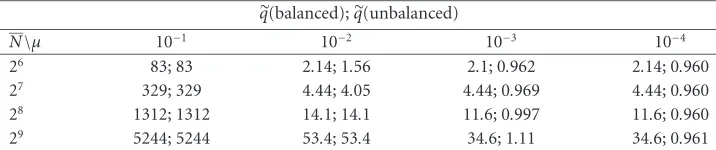
Figure 3.1. Fragment of the domain decomposition.

and (L−1) interfacial subdomainsϑl,l=1,...,L−1 (horizontal strips): ϑl=ωx_×ϑy

l = {0< x <1} ×

yb

l < y < yel

, ϑl−1∩ϑl= ∅, ρb

l =0≤x≤1, y=ylb, ρel =0≤x≤1, y=yle, yb

l < yl< yle, ρl0=∂ω∩∂ϑl.

(3.3)

Figure 3.1illustrates a fragment of the domain decomposition.

Onωml,m=1,...,M,l=1,...,L;θm,m=1,...,M−1 andϑl,l=1,...,L−1, intro-duce meshes:

ωh

ml=ωml∩ωh, θ h

m=θm∩ωh, ϑhl =ϑl∩ωh,

xb

m,xm,xemmM=1−1∈ωhx,

yb

l,yl,ylelL=1−1∈ωhy,

(3.4)

withωhx,ωhyfrom (2.1).

3.1. Statement of domain decomposition algorithm. We consider the following domain decomposition approach for solving (2.2). On each iterative step, we first solve problems on the nonoverlapping subdomainsωh_ml,m=1,...,M,l=1,...,Lwith Dirichlet bound-ary conditions passed from the previous iterate. Then Dirichlet data are passed from these subdomains to the vertical and horizontal interfacial subdomainsθhm,m=1,...,M−1 andϑhl,l=1,...,L−1, respectively. Problems on the vertical interfacial subdomains are computed. Then Dirichlet data from these subdomains are passed to the horizontal inter-facial subdomains before the corresponding linear problems are solved. Finally, we piece together the solutions on the subdomains.

Step 2. On subdomainsωh_ml,m=1,...,M,l=1,...,L, compute mesh functionsV_ml(n+1)(P) (here the indexnstands for a number of iterative steps) satisfying the following difference problems

ᏸh_+c∗_Z(n+1)

ml = −G(n)(P), P∈ωhml, G(n)_(P)≡ᏸh_V(n)_{+ fP,V}(n)_{, Z}(n+1)

ml (P)=0, P∈∂ωmlh , V(n+1)

ml (P)=V(n)(P) +Zml(n+1)(P), P∈ωhml.

(3.5)

Step 3. On the vertical interfacial subdomainsθhm,m=1,...,M−1, compute the diff er-ence problems

ᏸh_+c∗_Z(n+1)

m = −G(n)(P), P∈θmh,

Z(n+1) m (P)=

⎧ ⎪ ⎪ ⎪ ⎪ ⎨ ⎪ ⎪ ⎪ ⎪ ⎩

0, P∈γh0

m; Z(n+1)

ml (P), P∈γmhb∩ωhml,l=1,...,L; Z(n+1)

m+1,l(P), P∈γmhe∩ωhm+1,l,l=1,...,L, V(n+1)

m (P)=V(n)(P) +Zm(n+1)(P), P∈θ h m,

(3.6)

where we use the notation γh0

m =γ0m∩∂ωh, γhbm =γbm∩θhm, γhem =γem∩θhm. (3.7)

Step 4. On the horizontal interfacial subdomainsϑhl,l=1,...,L−1, compute the follow-ing difference problems

ᏸh_+c∗ _Z(n+1)

l = −G(n)(P), P∈ϑhl,

Z(n+1)

l (P)= ⎧ ⎪ ⎪ ⎪ ⎪ ⎪ ⎪ ⎪ ⎪ ⎨ ⎪ ⎪ ⎪ ⎪ ⎪ ⎪ ⎪ ⎪ ⎩

0, P∈ρhl0; Z(n+1)

ml (P), P∈ρhbl \θh∩ωhml,m=1,...,M; Z(n+1)

m,l+1(P), P∈

ρhe l \θh

∩ωh

m,l+1,m=1,...,M; Z(n+1)

m (P), P∈∂ϑh

l∩θhm,m=1,...,M−1,

V(n+1)

l (P)=V(n)(P) +Z(ln+1)(P), P∈ϑ h l,

(3.8)

where we use the notation

θh=

M−1

m=1

θhm, ϑh= L−1

l=1 ϑhl,

ρh0

l =ρ0l∩∂ωh, ρlhb=ρbl∩ϑ h

l, ρlhe=ρel∩ϑ h l.

Step 5. Compute the mesh functionV(n+1)_(P),P∈ωh_{by piecing together the solutions} on the subdomains

V(n+1)_(P)= ⎧ ⎪ ⎪ ⎪ ⎪ ⎨ ⎪ ⎪ ⎪ ⎪ ⎩

V(n+1)

ml (P), P∈ωhml\

θh∪ϑh; V(n+1)

m (P), P∈θhm\ϑ h

,m=1,...,M−1;

V(n+1)

l (P), P∈ϑ h

l,l=1,...,L−1.

(3.10)

Step 6. Stopping criterion: If a prescribed accuracy is reached, then stop; otherwise go to Step 2.

Algorithm (3.5)–(3.10) can be carried out by parallel processing. Steps2, 3, and 4 must be performed sequentially, but on each step, the independent subproblems may be assigned to different computational nodes.

Remark 3.1. We note that the original Schwarz alternating algorithm with overlapping subdomains is a purely sequential algorithm. To obtain parallelism, one needs a subdo-main colouring strategy, so that a set of independent subproblems can be introduced. The modification of the Schwarz algorithm (3.5)–(3.10) can be considered as an additive Schwarz algorithm.

3.2. Monotone convergence of algorithm (3.5)–(3.10). Additionally, we assume that f from (1.1) satisfies the two-sided constraints

0< c∗≤fu≤c∗, c∗,c∗=const. (3.11)

We say thatV(P) is an upper solution of (2.2) if it satisfies the inequalities

ᏸh_{V+f(P,V)≥0, P∈ω}h_{,V≥gon∂ω}h_{. (3.12)}

Similarly,V(P) is called a lower solution if it satisfies the reversed inequalities. Upper and lower solutions satisfy the following inequality

V(P)≤V(P), P∈ωh_{, (3.13)}

since by the definitions of lower and upper solutions and the mean-value theorem, for δV=V−V we have

ᏸh_{δV+fu(P)δV(P)≥0, P∈ω}h_,

δV(P)≥0, P∈∂ωh_, (3.14)

where fu(P)≡ fu[P,V(P) +Θ(P)δV(P)], 0<Θ(P)<1. In view of the maximum princi-ple inLemma 2.1, we conclude (3.13).

Theorem3.2. LetV(0)andV(0)be upper and lower solutions of (2.2), and let f(x,y,u) sat-isfy (3.11). Then the upper sequence{V(n)

}generated by (3.5)–(3.10) converges monotoni-cally from above to the unique solutionUof (2.2), and the lower sequence{V(n)_}generated by (3.5)–(3.10) converges monotonically from below toU:

V(0)_≤V(n)_≤V(n+1)_≤U≤V(n+1)_≤V(n)_≤V(0)_{, inω}h_{. (3.15)}

Proof. We consider only the case of the upper sequence. LetV(n)be an upper solution. Then by the maximum principle inLemma 2.1, from (3.5) we conclude that

Z(n+1)

ml (P)≤0, P∈ωhml,m=1,...,M,l=1,...,L. (3.16)

Using the mean-value theorem and the equation forZ_ml(n+1)(P), we obtain the difference equation forV_ml(n+1)

ᏸh_V(n+1)

ml +fP,Vml(n+1)= −c∗−fu(,nml)(P)

Z(n+1)

ml (P)≥0, P∈ωhml, f(n)

u,ml(P)≡fuP,V (n)

(P) +Θ(_mln)(P)Z_ml(n+1)(P), 0<Θ(_mln)(P)<1, V(n+1)

ml (P)=V (n)

(P), P∈∂ωh ml,

(3.17)

where nonnegativeness of the right-hand side of the difference equation follows from (3.11) and (3.16).

Taking into account (3.16) andV(n)is an upper solution, by the maximum principle inLemma 2.1, from (3.6) and (3.8) it follows that

Z(n+1)

m (P)≤0, P∈θ h

m,m=1,...,M−1,

Z(n+1)

l (P)≤0, P∈ϑ h

l,l=1,...,L−1.

(3.18)

Similar to (3.17), we obtain the difference problems forVm(n+1)

ᏸh_V(n+1)

m +fP,Vm(n+1)= −c∗−fu(,nm)(P) _Z(n+1)

m (P)≥0, P∈θmh,

V(n+1) m (P)=

⎧ ⎪ ⎪ ⎪ ⎪ ⎨ ⎪ ⎪ ⎪ ⎪ ⎩

g(P), P∈γh0 m; V(n+1)

ml (P), P∈γhbm ∩ωhml,l=1,...,L; V(n+1)

m+1,l(P), P∈γhem∩ωhm+1,l,l=1,...,L,

and forV_l(n+1) ᏸh_V(n+1)

l +fP,Vl(n+1)= −c∗−fu(,nl)(P) Z (n+1)

l (P)≥0, P∈ϑhl,

V(n+1)

l (P)= ⎧ ⎪ ⎪ ⎪ ⎪ ⎪ ⎪ ⎪ ⎨ ⎪ ⎪ ⎪ ⎪ ⎪ ⎪ ⎪ ⎩

g(P), P∈ρlh0; V(n+1)

ml (P), P∈

ρhb l \θh

∩ωh

ml,m=1,...,M; V(n+1)

m,l+1(P), P∈

ρhe l \θh

∩ωh

m,l+1,m=1,...,M; V(n+1)

m (P), P∈∂ϑhl ∩θ h

m,m=1,...,M−1,

(3.20)

where nonnegativeness of the right-hand sides of the difference equations follows from (3.11) and (3.18). Now we verify that the mesh functionV(n+1)defined by (3.10) is an up-per solution. From the boundary conditions forV_ml(n+1),Vm(n+1)andV_l(n), it follows that V(n+1)

satisfies the boundary condition in (2.2). Now from here, (3.17), (3.19), (3.20) and the definition ofV(n+1)in (3.10), we conclude that

G(n+1)_(P)=ᏸh_V(n+1)_{+ fP,V}(n+1)_{≥0, P∈ω}h_\γh_∪ρh_,

γhb,e

ml =xi=xbm,e,yel−1< yj< ylb, γhbm,e= L

l=1 γhb,e

ml , y0e=0, yLb=1,

γh₌M−1

m=1 γhb,e

m , ρh= L−1

l=1 ρhb,e

l .

(3.21)

To prove thatV(n+1)is an upper solution of problem (2.2), we have to verify only that the last inequality holds true on the interfacial boundariesγhb,e

ml andρhbl ,e,m=1,...,M−1, l=1,...,L−1.

We check this inequality in the case of the left interfacial boundaryγhb

ml, since the case withγhe

mlis checked in a similar way. From (3.5), (3.6), and (3.18), we conclude that the mesh functionW_ml(n+1)=V(n+1)

ml −Vm(n+1)satisfies the difference problem

ᏸh_+c∗_W(n+1)

ml =0, P∈θmlh =ωhml∩θmh, W(n+1)

ml (P)= ⎧ ⎨ ⎩

0, P∈γhb

ml=γmhb∩ωhml;

≥0, P∈∂θh ml\γhbml.

(3.22)

In view of the maximum principle inLemma 2.1, V(n+1)

ml (P)−Vm(n+1)(P)≥0, P∈θ h

ml. (3.23)

By (3.6),Vm(n+1)(P)=Vml(n+1)(P),P∈γhbml, and from (3.10) and (3.23), it follows that

−μ2_Ᏸ2

yVml(n+1)(P)= −μ2Ᏸ2yV(n+1)(P), P∈γmlhb,

−μ2_Ᏸ2

xVml(n+1)(P)≤ −μ2Ᏸx2V(n+1)(P), P∈γhbml.

Thus, using (3.17), we conclude G(n+1)_(P)≥ᏸh_V(n+1)

ml (P) +fP,Vml(n+1)≥0, P∈γmlhb. (3.25) Now we verify the inequalityG(n+1)_{(P)≥0 on the interfacial boundaryρ}hb

l , and the case withρhe_l is checked in a similar way. From (3.5), (3.8), (3.18), and (3.23), we conclude that the mesh functionW_ml(n+1)=V(n+1)

ml −Vl(n+1)satisfies the difference problem

ᏸh_+c∗ _W(n+1)

ml =0, P∈ϑhml=ωhml∩ϑhl,

W(n+1) ml (P)=

⎧ ⎨ ⎩

0, P∈ρhb_ml=xe

m−1< xi< xbm,yj=ylb

;

≥0, P∈∂ϑh ml\ρhbml.

(3.26)

By the maximum principle inLemma 2.1, V(n+1)

ml (P)−Vl(n+1)(P)≥0, P∈ϑ h

ml. (3.27)

By (3.8), V_l(n+1)(P)=V(n+1)

ml (P), P∈ρhbml∪ {(xem−1,ylb), (xbm,ylb)}, and from (3.10) and (3.27), it follows that

−μ2_Ᏸ2

xVml(n+1)(P)= −μ2Ᏸx2V(n+1)(P), P∈ρhbml,

−μ2_Ᏸ2

yVml(n+1)(P)≤ −μ2Ᏸ2yV(n+1)(P), P∈ρhbml.

(3.28)

Thus, using (3.17), we conclude G(n+1)_(P)≥ᏸh_V(n+1)

ml +f

P,V_ml(n+1)≥0, P∈ρhb_ml. (3.29)

From (3.6), (3.8), and (3.27), the mesh function ˆW_ml(n+1)=V(n+1)

m −V_l(n+1)satisfies the difference problem

ᏸh_+c∗ _W(n+1)

ml =0, P∈τmlh =θhm∩ϑhl,

W(n+1) ml (P)=

⎧ ⎨ ⎩

0, P∈ρhb,e

ml =xbm< xi< xem,yj=ybl,e;

≥0, P∈∂τh ml\

ρhb_ml∪ρhe_ml.

(3.30)

By the maximum principle inLemma 2.1, V(n+1)

m (P)−Vl(n+1)(P)≥0, P∈τhml. (3.31) By (3.8),V_l(n+1)(P)=V(n+1)

m (P),P∈ρhb_ml∪ {(xem,ylb), (xbm,ybl)}, and from (3.10) and (3.31), it follows that

−μ2_Ᏸ2_xV(n+1)

m (P)= −μ2Ᏸ2xV(n+1)(P), P∈ρhbml,

−μ2_Ᏸ2

yVm(n+1)(P)≤ −μ2Ᏸ2yV(n+1)(P), P∈ρhbml.

Thus, using (3.19), we conclude G(n+1)_(P)≥ᏸh_V(n+1)

m +fP,Vm(n+1)≥0, P∈ρhbml. (3.33) From here and (3.29), we conclude the required inequality onρhb_l \Pb,e

l ,Pbl,e= ∪Mm=1−1(xbm,e, yb

l). AtPbml=(xbm,ylb), we have V(n+1)

ml Pmlb =Vm(n+1)Pmlb =Vl(n+1)Pmlb , (3.34) and from (3.10), it follows that

−μ2_Ᏸ2_xV(n+1)_Pb

ml=− μ 2

b_xm

V(n+1)

m P_mlbx+−V_ml(n+1)P_mlb hb+

xm −

V(n+1) ml

Pb

ml

−V(n+1) ml

Pbx−

ml

hb_xm−

,

−μ2_Ᏸ2

yV(n+1)Pmlb =−μ 2

b yl

V(n+1)

l Pbyml+−Vml(n+1)Pmlb hb+

yl

−V

(n+1)

ml Pmlb −Vml(n+1)Pbyml− hb−

yl

,

Pbx±

ml =xbm±hxmb±,ybl, Pmlby±=xbm,ylb±hbyl±,

b

xm=2−1hxmb−+hbxm+, byl=2−1hylb−+hbyl+,

(3.35) wherehb+

xm,hbxm−are the mesh step sizes on the left and right fromPmlb , andhbyl+,hbyl−are the mesh step sizes on the top and bottom fromPb_ml. From here, (3.17), (3.23) and (3.27), we conclude

G(n+1)_(P)≥ᏸh_V(n+1)

ml +fP,Vml(n+1)≥0, P=Pbml. (3.36) With a similar argument for mesh pointP_le=(xem,ylb), we prove thatV(n+1)is an upper solution of problem (2.2) on the whole computational domainωh.

For arbitrary P∈ωh_{, it follows from (3.16), (3.18), and (3.13) that the sequence}

{V(n)

(P)} is monotonically decreasing and bounded below by V(P), where V is any lower solution. Therefore, the sequence is convergent and it follows from (3.5)–(3.8) that limZ_ml(n)=0, limZ_l(n)=0 and limZ_l(n)=0 asn→ ∞. Now by linearity of the operatorᏸh and the continuity of f, we have also from (3.5)–(3.8) that the mesh functionUdefined by

U(P)=_nlim

→∞V

(n)

(P), P∈ωh_{, (3.37)}

is an exact solution to (2.2). The uniqueness of the solution to (2.2) follows from esti-mate (2.8). Indeed, if by contradiction, we assume that there exist two solutionsU1and U2to (2.8), then by the mean-value theorem, the differenceδU=U1−U2satisfies the following difference problem

By (2.8),δU=0 which leads to the uniqueness of the solution to (2.2). This proves the

theorem.

Remark 3.3. Consider the following approach for constructing initial upper and lower solutionsV(0)andV(0). Suppose that a mesh functionR(P) is defined onωhand satisfies the boundary conditionR=gon∂ωh. Introduce the following difference problems

ᏸh_+c

∗Zν(0)=νᏸhR+f(P,R), P∈ωh,

Z(0)

ν (P)=0, P∈∂ωh,ν=1,−1.

(3.39)

Then the functionsV(0)=R+Z1(0),V(0)=R+Z (0)

−1 are upper and lower solutions, respec-tively. The proof of this result can be found in [4].

Remark 3.4. Since the initial iteration in algorithm (3.5)–(3.10) is either an upper or a lower solution, which can be constructed directly from the difference equation without any knowledge of the solution as we have suggested in the previous remark, this algorithm eliminates the search for the initial iteration as is often needed in Newton’s method. This gives a practical advantage in the computation of numerical solutions.

3.3. Convergence analysis of algorithm (3.5)–(3.10). We now establish convergence properties of algorithm (3.5)–(3.10).

If we denote

Z(n+1)_(P)=V(n+1)_(P)−V(n)_{(P), P∈ω}h_{, (3.40)}

then from (3.5)–(3.10),Z(n+1)_{can be written in the form}

Z(n+1)_(P)= ⎧ ⎪ ⎪ ⎪ ⎪ ⎨ ⎪ ⎪ ⎪ ⎪ ⎩

Z(n+1)

ml (P), P∈ωhml\

θh∪ϑh; Z(n+1)

m (P), P∈θhm\ϑ h

,m=1,...,M−1;

Z(n+1)

l (P), P∈ϑ h

l,l=1,...,L−1.

(3.41)

Introduce the following notation

b,e

xm=2−1hbxm−,e−+hbxm+,e+, byl,e=2−1hbyl−,e−+hbyl+,e+, (3.42)

wherehb_xm±,e±_{are the mesh step sizes on the left and right from pointsx}b,e

m andhbyl±,e±are the mesh step sizes on the top and bottom from pointsyb_l,e, and

κb

xm≡ μ 2

c∗b_xmhb+

xm, κ

e

xm≡ μ 2

c∗e_xmhe_xm−, qI=_1≤maxm≤M−1

κb xm;κexm, κb

yl≡ μ 2

c∗b_ylhb+ yl

, κeyl≡ μ

2

c∗e_ylhe−

yl, q

II_{= max} 1≤l≤L−1

κb

yl;κeyl.

Theorem3.5. For algorithm (3.5)–(3.10), the following estimate holds true _Z(n+1)

ωh≤q Z(n) _ωh, q=q+qI+qII, (3.44)

whereq=1−c∗/c∗.

Proof. Suppose that the sequence{V(n)_{}is generated by algorithm (3.5)–(3.10). Using} (2.8), from (3.5) we get the following estimate onZml(n+1)

_Z(n+1) ml ωh

ml≤ 1

c∗ G(n) ωh. (3.45) From here and (3.6) by (2.8), we conclude that

_Z(n+1) m _θh

m≤max

1

c∗ G(n) ωh; max_1≤l≤L Z (n+1) ml γhb

ml; Z (n+1) m+1,l γheml

≤_c1_∗ G(n) ωh,

γhb

ml=γmhb∩ωhml, γmlhe=γhem∩ωhm+1,l.

(3.46)

Similarly, from here and (3.8), we can obtain the estimate _Z(n+1)

l _ϑh l ≤

1

c∗ G(n) ωh. (3.47) Thus, by the definition ofZ(n+1)_{, we have}

_Z(n+1) ωh≤ 1

c∗ G(n) ωh. (3.48) From (3.17), (3.19) and (3.20) at the iterative stepn, and using the definition ofZ(n)_, we estimateG(n)_{as follows}

G(n)_{(P)= −c}∗_−f(n)

u (P)Z(n)(P), P∈ωh, ωh=ωh\γh∪ρh, (3.49) whereγh_andρh_{are defined in (3.21). By (3.11),}

1 c∗ G

(n)

ωh≤q Z(n) _ωh. (3.50) Now we estimateG(n)_onγh_{. Onγ}hb

ml= {xi=xbm,yle−1< yj< ybl}, we representG(n)in the form

G(n) _Pb

m=ᏸhVml(n)+f Pmb,Vml(n)− μ 2

b_xmhb+ xm

_V(n)

m Pmb+−Vml(n) Pmb+,

Pb

m=xbm,yj∈γmlhb, Pmb+=xbm+hbxm+,yj.

(3.51)

From (3.16) at the iterative stepnand the definition ofV(n)_{, we have} V(n)

From here, (3.17) and taking into account thatZ_ml(n)(P)=Z(n)_(P),P∈γhb

ml, we get the estimate

1

c∗ G(n) γhb ml≤

q+κbxm Z(n) ωh. (3.53)

Similarly, we can prove the estimate 1

c∗ G(n) γhe ml≤

q+κe_xm Z(n)

ωh. (3.54)

Thus, onγh_{, we conclude the estimate} 1 c∗ G

(n) γh≤

q+qI Z(n) _ωh. (3.55)

Onρhb_ml= {xe

m−1< xi< xbm,yj=ylb}, we representG(n)in the form G(n)_Pb

l=ᏸhVml(n)+fPlb,Vml(n)− μ 2

b ylhbyl+

V(n)

l Pbl+−Vml(n)Plb+, Pb

l =xi,ybl∈ρhbml, Plb+=xi,ylb+hbyl+.

(3.56)

From (3.16) at the iterative stepnand the definition ofV(n)_{, we have} V(n)

ml

Pb+ l

−V(n) l

Pb+

l

≤V(n−1)_Pb+ l

−V(n)_Pb+ l

= −Z(n)_Pb+ l

. (3.57)

From here and (3.17), and taking into account thatZ_ml(n)(P)=Z(n)_(P),P∈ρhb

ml, we get the estimate

1

c∗ G(n) ρhbml≤

q+κb_yl Z(n)

ωh. (3.58)

Similarly, we can prove the estimate 1

c∗ G(n) ρhe ml≤

q+κe_yl Z(n)

ωh. (3.59)

Onρhb_ml= {xbm< xi< xem,yj=ybl}, we representG(n)in the form

G(n)_Pb

l=ᏸhVm(n)+fPlb,Vm(n)− μ 2

b ylhbyl+

V(n)

l Pbl+−Vm(n)Plb+, Pb

l =

xi,yb_l∈ρhb_ml, P_lb+=xi,y_lb+hb_yl+.

(3.60)

From (3.18) at the iterative stepnand the definition ofV(n)_{, we have} V(n)

From here and (3.19), and taking into account thatZm(n)(P)=Z(n)_(P),P∈ρhb

ml, we get the estimate

1

c∗ G(n) ρhbml≤ _q

+κb_yl Z(n)

ωh. (3.62)

Similarly, we can prove the estimate 1

c∗ G(n) ρhe ml≤

q+κe_yl Z(n)

ωh. (3.63)

AtP_mlb =(x_mb,yb_l), we representG(n)_{in the form} G(n)_Pb

ml=ᏸhVml(n)+fPmlb ,Vml(n)

−_bμ2

xmhbxm+

V(n)

m Pmlbx+−Vml(n)Pbxml+

− μ2

b ylhbyl+ V

(n)

l Pbyml+−Vml(n)Pbyml+, Pbx+

ml =

xb

m+hbxm+,ylb

, P_mlby+=xb

m,ybl+hbyl+

.

(3.64)

From (3.16) at the iterative stepnand the definition ofV(n)_{, we have} V(n)

mlPbxml+−Vm(n)Pbxml+≤V(n−1)Pmlbx+−V(n)Pbxml+

= −Z(n)_Pbx+ ml

, V(n)

mlPmlby+−Vl(n)Pmlby+≤V(n−1)Pmlby+−V(n)Pmlby+

= −Z(n)_Pby+ ml .

(3.65)

From here and (3.17), and taking into account thatZ_ml(n)(P_mlb )=Z(n)_(Pb

ml), we get the esti-mate

1 c∗G(n)

Pb

ml≤

q+κbxm+κbyl Z(n) ωh. (3.66)

By the same reasonings, the following estimate holds true 1

c∗G(n) _Pe

m−1,l≤q+κxe,m−1+κbyl Z(n) ωh, P_me_−1,l=xe_m−1,yb_l. (3.67) Onρhb_l , we conclude the estimate

1 c∗ G

(n) ρhb

l ≤

q+qI+qII Z(n) _ωh. (3.68)

The same estimate holds true onρhe_l , and onρhwe get the estimate 1

c∗ G(n) ρh≤

From here, (3.50) and (3.55), we conclude the estimate 1

c∗ G(n) ωh≤

q+qI+qII Z(n)

ωh. (3.70)

and, using (3.48), we prove the theorem.

Remark 3.6. For the undecomposed algorithm, withM=1 andL=1, one hasωh=ωh in (3.50) which together with (3.48) gives estimate (3.44) withq=q.

Without loss of generality, we assume that the boundary condition in (1.1) is zero, that is,g(P)=0. This assumption can always be obtained via a change of variables. Let the initial functionV(0)_{be chosen in the form of (3.39) withR(P)=0, that is,V}(0)_{is the} solution of the following difference problem

ᏸh_+c

∗V(0)=νf(P, 0), P∈ωh,

V(0)_{(P)=0, P∈∂ω}h_{, ν=1,−1.} (3.71)

Then the functionsV(0)(P),V(0)(P) corresponding toν=1 andν= −1 are upper and lower solutions, respectively.

Theorem3.7. Let the factorqin (3.44) satisfy the conditionq < 1. Suppose that the initial upper or lower solutionV(0)_{is chosen in the form of (3.71). Then for algorithm (3.5)–(3.10),} the following estimate holds true

_V(n)_−U

ωh≤ c0(q)

n

(1−q) f(P, 0) ωh, c0=

3c∗+c∗

c∗c∗ , (3.72)

whereUis the solution to (2.2).

Proof. Using (3.44), we have _V(n+k)_−V(n)

ωh≤

n+k−1

i=n

_V(i+1)_−V(i) ωh=

n+k−1

i=n

_Z(i+1) ωh

≤ q

1−q Z(n) ωh≤ (q)

n

1−q Z(1) ωh.

(3.73)

Taking into account that limV(n+k)_{=U ask→ ∞, whereUis the solution to (2.2), we} conclude the estimate

_V(n)_−U

ωh≤ (q)

n

1−q Z(1) ωh. (3.74) From (3.48), (3.71) and the mean-value theorem

_Z(1) ωh≤ 1

c∗ G(0) ωh≤ 1

c∗ ᏸhV(0) ωh+ 1 c∗ f

_P ,V(0)

ωh

≤_c1_∗c∗ V(0) ωh+ f(P, 0) _ωh+ 1

c∗ f(P, 0) ωh+ V(0) _ωh.

From here and estimatingV(0)_{from (3.71) with (2.8), V}(0)

ωh≤ 1

c∗

_{f(P, 0) ω}h, (3.76)

we conclude the estimate onZ(1)_{in the form Z}(1)

ωh≤c₀ f(P, 0) _ωh, (3.77)

wherec0is defined in (3.72). Thus, from here and (3.74), we prove (3.72). Remark 3.8. In the next section, we present sufficient conditions to guarantee the in-equalityq < 1 required inTheorem 3.7.

3.4. Uniform convergence of the monotone domain decomposition algorithm (3.5)– (3.10). Here we analyze a convergence rate of algorithm (3.5)–(3.10) applied to the dif-ference scheme (2.2) defined on the piecewise uniform mesh introduced in [7]. On this mesh, the difference scheme (2.2) convergesμ-uniformly to the solution of (1.1).

The piecewise uniform mesh is formed in the following manner. We divide each of the intervalsωx=[0, 1] andωy=[0, 1] into three parts each [0,σx], [σx, 1−σx], [1−σx, 1], and [0,σy], [σy, 1−σy], [1−σy, 1], respectively. Assuming thatNx,Nyare divisible by 4, in the parts [0,σx], [1−σx, 1] and [0,σy], [1−σy, 1] we use a uniform mesh withNx/4 + 1 and Ny/4 + 1 mesh points, respectively, and in the parts [σx, 1−σx], [σy, 1−σy] with Nx/2 + 1 andNy/2 + 1 mesh points, respectively. This defines the piecewise equidistant mesh in thex- andy-directions condensed in the boundary layers atx=0, 1 andy=0, 1:

xi=

⎧ ⎪ ⎪ ⎪ ⎨ ⎪ ⎪ ⎪ ⎩

ihxμ, i=0, 1,...,Nx/4; σx+i−Nx/4hx, i=Nx/4 + 1,..., 3Nx/4; 1−σx+i−3Nx/4hxμ, i=3Nx/4 + 1,...,Nx,

yj=

⎧ ⎪ ⎪ ⎪ ⎨ ⎪ ⎪ ⎪ ⎩

jhyμ, j=0, 1,...,Ny/4; σy+j−Ny/4hy, j=Ny/4 + 1,..., 3Ny/4; 1−σy+j−3Ny/4hyμ, j=3Ny/4 + 1,...,Ny,

(3.78)

wherehxμ,hyμandhx,hyare the step sizes inside and outside the boundary layers, respec-tively. The transition pointsσx, (1−σx) andσy, (1−σy) are determined by

σx=min4−1,μc∗−(1/2)lnNx, σy=min4−1,μc∗−(1/2)lnNy. (3.79)

assume that

σx=μc−(1/2)

∗ lnNx, hxμ=4μc∗−(1/2)Nx−1lnNx, Nx−1< hx<2Nx−1, σy=μc−(1/2)

∗ lnNy, hyμ=4μc−(1∗ /2)Ny−1lnNy, Ny−1< hy<2Ny−1.

(3.80)

The difference scheme (2.2) on the piecewise uniform mesh (3.80) convergesμ -uni-formly to the solution of (1.1):

max P∈ωh

_{U(P)−u(P)≤C}

N−1_lnN2_{, N=minNx,Ny, (3.81)}

where constantCis independent ofμandN. The proof of this result can be found in [7]. Theorem3.9. Let the interfacial subdomainsθhm,m=1,...,M−1andϑhl,l=1,...,L−1 be located in thex- andy-directions, respectively, outside the boundary layers. Assumeμ≤

μ01, and the following condition

N≤α

c∗/2

μ0 , N=max

Nx,Ny, 0< α <1,α=const. (3.82)

If the initial upper or lower solutionV(0)_{is chosen in the form of (3.71), then the} mono-tone domain decomposition algorithm (3.5)–(3.10) on the piecewise uniform mesh (3.80) convergesμ-uniformly to the solution of the problem (1.1):

_V(n)_−u

ωh≤CN−1lnN2+ c0(Q)

n

(1−Q)

_{f(P, 0) ω}h,

Q=1−1−α2_cc∗_∗<1, c0=3c∗+c ∗ c∗c∗ ,

(3.83)

where constantCand the factorQare independent ofμandN.

Proof. Under the above assumption onN, the factorqin (3.44) satisfies the condition

q <1. Indeed, since the interfacial subdomains are located outside the boundary layers, where the step sizeshx andhy are in use, then using (3.80),qI andqII from (3.44) are estimated as follows

qI₌ μ2 c∗_h2

x <

μ0N 2

c∗ , qII= μ2 c∗_h2

y <

μ0N 2

c∗ . (3.84)

Thus,q < Q < 1, and we can applyTheorem 3.7. From here, (3.72) and (3.81), we

Remark 3.10. Such domain decompositions, in which the interfacial subdomains are out-side the boundary layers, are said to beunbalanced, since the distribution of mesh points among the nonoverlapping main subdomains is uneven. By contrast, abalanceddomain decomposition is one in which the mesh points are equally distributed among the main subdomains. For balanced decompositions, the first and last interfacial subdomains each overlap the boundary layer.

4. Monotone domain decomposition algorithm for the parabolic problem (1.2)

For solving the nonlinear difference scheme (2.5), we construct and investigate a paral-lel domain decomposition algorithm based on the domain decomposition of the spatial domainωintroduced inSection 3.

4.1. Statement of domain decomposition algorithm for solving (2.5). On each time levelt∈ωτ_{, we calculaten}

∗iteratesV(n)(P,t),P∈ωh,n=1,...,n∗as follows.

Step 1. Initialization: on the meshωh, chooseV(0)_(P,t),P∈ωh_{satisfying the boundary} conditionV(0)_{(P,t)=g(P,t) on∂ω}h_.

Forn=0ton∗−1do Steps2–5

Step 2. On subdomainsωh_ml,m=1,...,M,l=1,...,L, compute mesh functionsV_ml(n+1)(P, t),m=1,...,M,l=1,...,Lsatisfying the following difference problems

ᏸhτ_+c∗_Z(n+1)

ml = −G(n)(P,t), P∈ωhml, G(n)_(P,t)≡ᏸhτ_V(n)_{(P,t) +fP,t,V}(n)_−τ−1_V(P,t−τ),

Z(n+1)

ml (P,t)=0, P∈∂ωhml, V(n+1)

ml (P,t)=V(n)(P,t) +Zml(n+1)(P,t), P∈ωhml.

(4.1)

Step 3. On the vertical interfacial subdomainsθhm,m=1,...,M−1, compute the diff er-ence problems

ᏸhτ_+c∗_Z(n+1)

m = −G(n)(P,t), P∈θmh,

Z(n+1) m (P,t)=

⎧ ⎪ ⎪ ⎪ ⎪ ⎨ ⎪ ⎪ ⎪ ⎪ ⎩

0, P∈γh0

m; Z(n+1)

ml (P,t), P∈γhbm ∩ωhml,l=1,...,L; Z(n+1)

m+1,l(P,t), P∈γhem∩ωhm+1,l,l=1,...,L, V(n+1)

m (P,t)=V(n)(P,t) +Zm(n+1)(P,t), P∈θhm,

(4.2)

Step 4. On the horizontal interfacial subdomainsϑhl,l=1,...,L−1, compute the follow-ing difference problems

ᏸhτ_+c∗ _Z(n+1)

l = −G(n)(P,t), P∈ϑhl,

Z(n+1)

l (P,t)= ⎧ ⎪ ⎪ ⎪ ⎪ ⎪ ⎪ ⎪ ⎪ ⎨ ⎪ ⎪ ⎪ ⎪ ⎪ ⎪ ⎪ ⎪ ⎩

0, P∈ρh0

l ; Z(n+1)

ml (P,t), P∈ρlhb\θh∩ωhml,m=1,...,M; Z(n+1)

m,l+1(P,t), P∈

ρhe l \θh

∩ωh

m,l+1,m=1,...,M; Z(n+1)

m (P,t), P∈∂ϑh

l∩θhm,m=1,...,M−1,

V(n+1)

l (P,t)=V(n)(P,t) +Zl(n+1)(P,t), P∈ϑ h l,

(4.3)

where we use the notation from (3.8).

Step 5. Compute the mesh functionV(n+1)_(P,t),P∈ωh_{by piecing together the solutions} on the subdomains

V(n+1)_(P,t)= ⎧ ⎪ ⎪ ⎪ ⎪ ⎨ ⎪ ⎪ ⎪ ⎪ ⎩

V(n+1)

ml (P,t), P∈ωhml\

θh∪ϑh; V(n+1)

m (P,t), P∈θhm\ϑ h

,m=1,...,M−1;

V(n+1)

l (P,t), P∈ϑ h

l,l=1,...,L−1.

(4.4)

Step 6. Set up

V(P,t)=V(n∗)_{(P,t), P∈ω}h_{. (4.5)}

4.2. Monotone convergence of algorithm (4.1)–(4.5). Additionally, we assume that f from (1.2) satisfies the two-sided constraints

0≤fu≤c∗_{, c}∗_{=const. (4.6)}

On a time levelt∈ωτ_{, we say thatV(P,t) is an upper solution with respect to a given} functionV(P,t−τ) if it satisfies

ᏸhτ_{V(P,t) +fP,t,V−τ}−1_{V(P,t−τ)≥0, P∈ω}h_,

V(P,t)≥g(P,t), P∈∂ωh_. (4.7) Similarly,V(P,t) is called a lower solution with respect toV(P,t−τ) if it satisfies the reversed inequalities. On each time level, upper and lower solutions satisfy the following inequality

V(P,t)≤V(P,t), P∈ωh_{. (4.8)} The proof of this result is similar to that of (3.13).

Theorem4.1. LetV(P,t−τ)be given andV(0)(P,t),V(0)(P,t)be upper and lower solu-tions corresponding toV(P,t−τ). Suppose that f satisfies (4.6). Then the upper sequence

{V(n)

(P,t)}generated by (4.1)–(4.5) converges monotonically from above to the unique so-lutionᐂ(P,t)of the problem

ᏸhτ_{V(P,t) +f(P,t,V)−τ}−1_{V(P,t−τ)=0, P∈ω}h_,

V(P,t)=g(P,t), P∈∂ωh_, (4.9)

and the lower sequence{V(n)_{(P,t)}generated by (4.1)–(4.5) converges monotonically from} below toᐂ(P,t):

ᐂ(P,t)≤V(n+1)

(P,t)≤V(n)

(P,t)≤V(0)

(P,t), P∈ωh_,

V(0)_(P,t)≤V(n)_(P,t)≤V(n+1)_{(P,t)≤ᐂ(P,t), P∈ω}h_. (4.10)

Proof. The proof of the theorem is similar to the proof ofTheorem 3.2and based on the maximum principle inLemma 2.1and the estimate (2.8) with β=1 for the difference

operatorᏸhτ.

Remark 4.2. In the case of algorithm (4.1)–(4.5), Remarks3.1–3.4hold still true at each time stept∈ωτ_{. We only mention that the difference problem in (3.39) becomes}

ᏸhτ_Z(0)

ν =νᏸhτR(P,t) + f(P,t,R)−τ−1V(P,t−τ), P∈ωh,

Z(0)

ν (P,t)=0, P∈∂ωh,ν=1,−1.

(4.11)

4.3. Convergence analysis of algorithm (4.1)–(4.5). We now establish convergence properties of algorithm (4.1)–(4.5).

Introduce the following notation

υb

xm≡ μ

2

c∗_+τ−1b_xmhb+

xm, υ

e

xm≡ μ

2

c∗_+τ−1e_xmhe_xm−, υb

yl≡ μ

2

c∗_+τ−1b_ylhb+ yl

, υe_yl≡ μ2

c∗_+τ−1e ylheyl−, rI_{= max}

1≤m≤M−1 _υb

xm;υexm, rII= max 1≤l≤L−1

_υb yl;υeyl,

(4.12)

where all the step sizes are defined in (3.42).

Similar toTheorem 3.5, on each time levelt∈ωτ_{, we have the following convergence} property of algorithm (4.1)–(4.5).

Theorem4.3. For algorithm (4.1)–(4.5), the following estimate holds true _Z(n+1)_(t)

ωh≤r Z(n)(t) _ωh, r=r+rI+rII,t∈ωτ, (4.13)

Proof. The proof of the theorem is similar to the proof ofTheorem 3.5and based on the maximum principle inLemma 2.1and the estimate (2.8) with β=1 for the difference

operatorᏸhτ.

Remark 4.4. In similar fashion to the proof ofTheorem 3.5, the proof ofTheorem 4.3 includes the resultr=rfor the undecomposed algorithm.

Without loss of generality, we assume that for the parabolic problem (1.2), the bound-ary conditiong(P,t)=0. This assumption can always be obtained via a change of vari-ables. Let on each time level the initial functionV(0)_{(P,t) be chosen in the form of (4.11)} withR(P,t)=0, that is,V(0)_{(P,t) is the solution of the following difference problem}

ᏸhτ_V(0)_{(P,t)=νf(P,t, 0)−τ}−1_{V(P,t−τ), P∈ω}h_,

V(0)_{(P,t)=0, P∈∂ω}h_{, ν=1,−1.} (4.14)

Then the functionsV(0)(P,t),V(0)(P,t) corresponding toν=1 andν= −1 are upper and lower solutions, respectively.

Theorem4.5. In the domain decomposition algorithm (4.1)–(4.5), letV(0)_{(P,t)be chosen} in the form of (4.14), and let f satisfy (4.6). Suppose that on each time level, the number of iteratesn∗satisfiesn∗≥2. Then the following estimate on convergence rate holds

max tk∈ωτ

_V

tk−Utk ≤Dc∗_+η(r)n∗−1_,

η=c∗_+τ−1_rI_+rII_, (4.15)

wherer, rI _andrII _{are defined inTheorem 4.3,U(P,t)is the solution to (2.5) and} con-stantDis independent ofμandτ. Furthermore, on each time level the sequence{V(n)_(P,t)} converges monotonically.

Proof. The difference problem forV(P,tk)=V(n∗)_{(P,tk) can be represented in the form}

ᏸhτ_{VP,tk+ fP,tk,V−τ}−1_VP,tk

−1=G(n∗)P,tk, P∈ωh,

VP,tk=gP,tk, P∈∂ωh_. (4.16)

From here, (2.5) and using the mean-value theorem, we get the difference problem for W(P,tk)=V(P,tk)−U(P,tk)

ᏸhτ_{+ f}(n∗)

u WP,tk=G(n∗)P,tk+τ−1WP,tk−1, P∈ωh,