Performance analysis on joint channel decoding and state estimation in cyber physical systems

cyber-physical systems

Liang Li

, Shuping Gong

, Ju Bin Song

and Husheng Li

Abstract

We propose to use an mean square error (MSE) transfer chart to evaluate the performance of the proposed belief propagation (BP)-based channel decoding and state estimation scheme. We focus on two models to evaluate the performance of BP-based channel decoding and state estimation: the sequential model and the iterative model. The numerical results show that the MSE transfer chart can provide much insight about the performance of the proposed channel decoding and state estimation scheme.

Keywords: Channel coding, State estimation, EXIT chart, MSE transfer chart, CPSs

1 Introduction

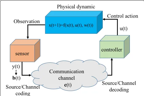
Communication has been of great importance in cyber-physical systems (CPSs), which sends observations of the physical dynamics from the sensor to the controller as illustrated in Fig. 1. One promising way to improve the performance of physical dynamics (or system state) esti-mation is the BP-based joint channel decoding and sys-tem state estimation algorithm, which we have already developed in [1] to utilize time-domain redundancy of system state to assist channel decoding. For example, the quantized codeword before source/channel encoding at discrete timet, denoted asb(t), is generated by the obser-vation of the physical dynamics, denoted asy(t), wheret

can be viewed as the beginning oftth time slot. Due to the time correlation of the system states, the observation

y(t)is correlated withy(t−1), thus,b(t−1)can provide some information for decoding the quantized codeword, i.e., b(t) in discrete time t. Even though the effective-ness of the proposed joint channel decoding and system state estimation algorithm has been verified by numeri-cal results in [1], the procedure of the given algorithm is still left unspecified. Contributing toward the previous work, this paper addresses the procedure of the message

*Correspondence: [email protected]

1_{Department of Electrical Engineering and Computer Science, the University} of Tennessee, Knoxville, Knoxville, USA

Full list of author information is available at the end of the article

passing between the channel decoder, which processes the information of quantized bits, and the state estimator, which handles the information of continuous state values. We analyze the proposed algorithm from the following perspectives:

• Does the proposed algorithm converge and help to improve channel decoding and system state estimation?

• How much gain can be obtained by using redundancy of observations in time domain to assist channel decoding?

As pointed out before, the CPS is a hybrid system [2], which consists of system statex(t), observationy(t)with continuous values, and information bits b(t) transmit-ted in wireless communication with discrete values. The challenges in the channel decoding and system state esti-mation framework are that the priori inforesti-mation trans-mitted from a state estimator to a channel decoder is the prediction of y(t), while the channel decoder actu-ally requires the priori information of each quantized bit ofy(t), and that the output of the channel decoder is the extrinsic information of each quantized bit ofy(t), while the state estimator actually requires the estimation ofy(t)

from the channel decoder. To handle these challenges, two models, the BP-based sequential model and the BP-based iterative model, are given to evaluate the performance of BP-based channel decoding and system state estimation

Fig. 1An illustration of the components in CPSs

framework. The former can be used to evaluate the per-formance of system state estimation over multiple time slots, e.g., the gain by utilizing priori information from the previous time slot to assist channel decoding and state estimation at the current time slot. The latter can be used to check the following points:

1. Does the iterative channel decoding and estimation converge, and how many iterations are sufficient? 2. How much gain can be obtained by utilizing priori

information from the previous time slots to assist state estimation at the current time slot?

In the area of wireless communication, the purpose of performance analysis for decoding scheme is to find out if, for any given encoder, decoder, and channel noise power, a message-passing iterative decoder can correct the errors or not.

To analyze the performance, in [3–5], Ten Brink pro-posed using an extrinsic information transfer (EXIT) chart to track the iterative decoding performance. Based on the assumption that the distribution of the extrinsic log-likelihood ratios (LLRs) is a Gaussian distribution, the EXIT chart tracks mutual information from the extrinsic LLRs through an iterative decoding process. Compared with the previously used method of density evolution, the EXIT chart is computationally simplified, and it also allows to visualize the evolution of mutual information through iterative decoding process in a graph. The details of the EXIT chart can be found in [6].

The EXIT chart has two useful properties as shown in [7]. One is the necessary condition for the convergence of iterative decoding that the flipped EXIT chart curve of the outer decoder for iterations lies below the EXIT chart curve of the inner coder. The other is that the area under the EXIT curve of outer code relates to the rate of inner coder. In [8], the authors demonstrated that if the priori channel is an erasure channel, for any outer code

of rateR, the area under the EXIT curve is 1−R. To our best knowledge, the area property of the EXIT chart has been proved only for cases where the priori channels are erasure channels.

The mean square error (MSE) transfer chart improves the EXIT chart as shown in [7], because the area property of the MSE transfer chart corresponding to the area prop-erty of the EXIT charts has been proven in both erasure channels and AWGN channels. Instead of tracking mutual information, the MSE transfer chart, as an alternative to evaluate decoding performance, has been proposed in [9] to track the iterative decoding performance based on the relationship between mutual information and the mini-mum mean square error (MMSE) for the additive white Gaussian noise (AWGN) channel.

In this paper, we use the MSE transfer chart to ana-lyze the message passing procedure of channel decoding and system state estimation by assuming that the priori information is an AWGN channel. Compared with [9], our hybrid model prioritizes practicality because the system states and observations considered are continuous values while the information transmitted in wireless system are quantized information bits. Unlike previous research, our algorithm addresses the message passing between con-tinuous values from the state estimator and quantized information bits from the channel decoder with the condi-tion that the system state is correlated over different time slots. In addition, in order to view the evolution of the estimation error, we analyze the performance of state esti-mation in two cases: within two time slots and more than two time slots.

the performance evaluation of iterative channel decoding. Section 3 describes the system models for performance analysis. Section 4 presents the message passing frame-work between system observation and channel decoding. Section 5 describes the MSE transfer chart, and Section 6 presents how to use the MSE transfer chart to evaluate BP-based sequential and iterative channel decoding and state estimation. Finally, a brief conclusion is given in Section 7.

2 Preliminaries on the EXIT Chart

In this section, we review the concept of the EXIT chart and the MSE transfer chart by iterative decoding the out-put of a serially concatenated encoder. In Section 2.1, we use an example to illustrate the serially concatenated cod-ing scheme and its iterative decodcod-ing process. Then, in Section 2.2, we review how to use the EXIT chart and the MSE transfer chart to analyze the performance of iterative decoding.

2.1 A serially concatenated encoding scheme and corresponding iterative decoding algorithm

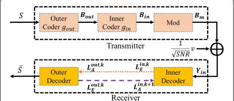
Figure 2 shows a simple serially concatenated encoding scheme and its corresponding iterative decoding scheme.

At the transmitter, the sourceSwith binary values is a vector with the lengthLs, i.e.,S=[S1,···,SLs].Sis encoded by the outer channel encoder, which is a systematic convo-lutional encoder whose generator isgoutwith an output of

Bout, a vector with the lengthLout. Next,Boutis encoded by the inner channel encoder, also a systematic convolu-tional encoder whose the generator isginwith an output of

Bin, a vector with the lengthLin. Finally,Binis modulated with an output ofBm, i.e.,Bm,i=2Bin,i−1,i=1,· · ·,Lin, and then sent over an AWGN channel with an output that can be calculated by

Fig. 2A demo of concatenated encoding and iterative decoding

Yin priori information from the outer decoder, i.e., Lin,k_A =

Lout,k_E −1, whereLout,k_E −1is the extrinsic information of the

outer decoder from (k −1)th decoding round, and the output for it isLin,k_E , i.e.,

Lin,k_E,i =LLRSi|Yin,Lin,kA,i,gin

i=1,· · ·,Ls (2)

where Lin,k_A,i means the priori information ofLin,k_A,i for all

SexceptSi. The input for the outer channel decoder is a priori information from the inner decoder, i.e., Lout,k_A = Lin,k_E , and the output for it isLout,k_E , i.e.,

whereLout,k_A,i means the priori information ofLout,k_A,i for all

SexceptSi.

2.2 The EXIT chart and the MSE transfer chart

The iterative decoding scheme in [30] can be analyzed by tracking the density evolution over iterations. However, the density evolution is complex as it requires to obtain probability density function (PDF) of extrinsic LLRs for each iteration; in addition, it does not provide much insight about the operations of iterative decoding. In order to overcome the drawbacks of density evolution, many transfer chart-based analysis frameworks have been pro-posed, such as the EXIT chart by [3–5] and the MSE transfer chart by [9]. The idea of these transfer chart-based analysis frameworks is to approximate the PDF of extrinsic LLRs exchanged between the inner decoder and outer decoder by a parameter, i.e.,

F(S,L)= 1

The measure used by the EXIT chart is mutual informa-tion, i.e.,F(S,L)=I(S,L), which is based on the observa-tion that the PDF of extrinsic LLRs can be approximated by a Gaussian distribution [3–5].

ofSbased on observationYin[9], i.e.,

The EXIT chart and the MSE transfer chart-based decoding frameworks for a serially concatenated encod-ing scheme are shown in Fig. 3 (a and b), respectively. The transfer chart includes two transfer curves. One curve is the measure for the priori information of inner decoder, i.e.,F_Ain(S,L), versus the measure for the extrinsic infor-mation of inner decoder, i.e.,F_Ein(S,L); the other curve is the measure for the priori information of outer decoder, i.e.,F_Aout(S,L), versus the measure for the extrinsic infor-mation of outer decoder, i.e.,F_Eout(S,L). The EXIT chart and the MSE transfer chart for the serially concatenated coding scheme are shown in Figs. 4 and 5, respectively. The predicted decoding path is also shown in these two figures. Since there is a decoding path found between the two curves, the iterative decoding converges.

3 System model

In this section, we describe the system model for the analysis.

3.1 Linear dynamic system and communication system We consider a discrete time linear dynamic system, whose state evolution is given by

x(t+1) = Ax(t)+Bu(t)+n(t)

y(t) = Cx(t)+w(t) (6)

wherex(t)is theN-dimensional vector of system state at time slott,u(t)is theM-dimensional control vector,y(t)is theK-dimensional observation vector, andn(t)andw(t)

are noise vectors, which are assumed to be Gaussian dis-tributions with zero mean and covariance matrixnand w, respectively. For simplicity, we do not consideru(t).

Additionally, we assume that the observation vectory(t)

is obtained by a sensor1, and the sensor quantizes each dimension of the observation vectory(t)usingBbits, thus forming aKB-dimensional binary vector, which is given by

b(t)=(b1(t),b2(t),. . .,bKB(t)) (7)

The information bitsb(t)are then put into an encoder to generate a codeword c(t). Suppose that the binary phase-shift keying (BPSK) is used for the transmission between the sensor and the controller, and c(t) is con-verted to alphabet{−1,+1}withs(t)=2c(t)−1. Next, the sequence s(t)is passed through a modulator and trans-mitted into an AWGN channel. Then, the received signal at the controller is given by

r(t)=s(t)+e(t) (8)

where the additive white Gaussian noisee(t) has a zero expectation and variance c. Note that we consider the AWGN channel, ignore the fading and normalize the transmit power to be 1. The algorithm and conclusion in this work can be easily extended to the cases with different channels and different types of fading.

3.2 Models for belief propagation based channel decoding and state estimation

In this section, we firstly introduce the Bayesian network structure and then use the following two models to eval-uate BP-based channel decoding and state estimation: BP-based sequential processing and BP-based iterative processing.

3.2.1 Bayesian network structure and the message passing

The Bayesian network structure of the dynamic system and communication system is shown in Fig. 6, where the

Fig. 4An example of the EXIT chart for concatenated encoding and iterative decoding,gout=gin=[ 1, 1, 0, 1; 1, 0, 0, 1] , SNR= −2 dB

message passing in the system is illustrated by dotted arrows and dashed arrows in the figure with three time slots:x(t−2),x(t−1), andx(t). The dashed arrows trans-mitπ-message from a parent to its children in Pearl’s BP, and the details and formal description can be found in [31]. For instance, the message passed fromx(t−2) to

x(t−1)isπx(t−2),x(t−1)(x(t−2)), which is the priori infor-mation ofx(t−2)given that all the informationx(t−2) has been received. The dotted arrows transmitλ-message from a child to its parent. For instance, the message passed fromx(t−1)tox(t−2)isλx(t−1),x(t−2)(x(t−2)), which is

the likelihood ofx(t−2)given that the informationx(t−1) has been received.

Note that theπ-message andλ-message are passing in the form of probability distribution function (PDF), and based on the Bayesian network structure in Fig. 6 and Pearl’s BP, the updating order and the message passing in one iteration is given as follows: step 1:x(t−1)→y(t−1); step 2:y(t−1)→b(t−1); step 3:b(t−1) →y(t−1); step 4:y(t−1) →x(t−1); step 5:x(t−1) →x(t); step 6:x(t) → y(t); step 7:y(t) → b(t); step 8:b(t) → y(t); step 9:y(t)→x(t); step 10:x(t)→x(t−1); and step 11:

Fig. 6Bayesian network structure and the message passing for CPSs

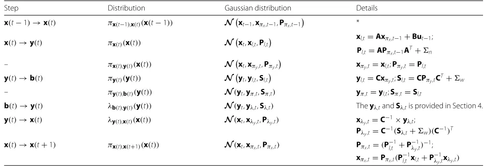
x(t−1)updates information. The key steps in the Pearl’s BP have be derived as shown in Table 1, where the PDF of λb(t),y(t)(y(t))will be computed by iterative decoding provided in Section 4.

3.2.2 Model for BP-based sequential processing

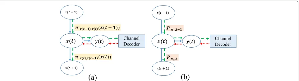
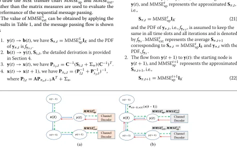
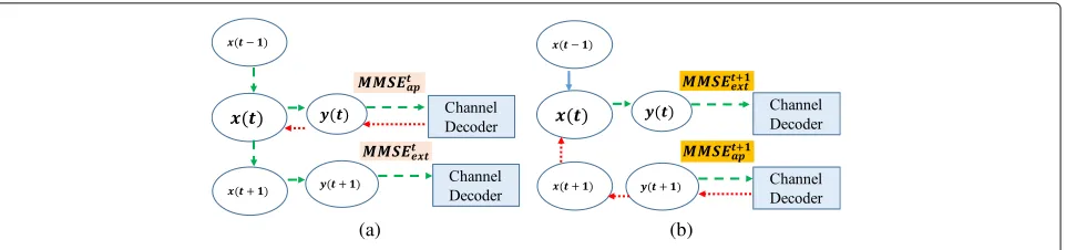
Based on the Bayesian network structure in Fig. 6, we use the framework as shown in Fig. 7 (a) to evaluate sequential channel decoding and state estimation over more than two time slots. The priori information from the time slot t−1, i.e.,πx(t−1),x(t)(x(t−1)), is used to assist channel decoding and state estimation at the time slott, i.e., the estimated distribution ofx(t−1), and we assume that it is also a Gaussian distribution with mean xπx,t−1and covariance matrixPπx,t−1, i.e.,N(xt−1,xπx,t−1,Pπx,t−1).

As noted in Section 1, two objectives here are to evaluate how much gain can be obtained by utilizing πx(t−1),x(t)(x(t−1))to assist channel decoding and state estimation at time slot t and to evaluate the perfor-mance of state estimation over multiple time slots, i.e., the evolution ofPπx,t−1as shown in Fig. 7(b).

3.2.3 Model for BP-based iterative processing between two

time slots

Figure 8(a) illustrates the model used to evaluate BP-based iterative channel decoding and state estimation between

two time slots. The inputs for this model include the received signals at the controller within the two time slots, i.e.,r(t)andr(t+1), which can be found in Fig. 6, and the priori information from the previous time slott−1, i.e., πx(t−1),x(t)(x(t−1)).

The goal is to evaluate the performance of iterative channel decoding and state estimation for different real-izations of the two distributions forπx(t−1),x(t)(x(t−1)). For instance, when πx(t−1),x(t)(x(t − 1)) (say, Pπx,t−1) equals to 0×I,x(t−1)is a determined state estimation. Therefore, this reference model can be converted to the model shown in Fig. 8 (b) by settingπx(t−1),x(t)(x(t−1) (say,Pπx,t−1) as 0×I. Or ifπx(t−1),x(t)(x(t−1))(say,Pπx,t−1) is set as∞ ×I,x(t−1)is unknown. Then, the reference model is transformed to the model shown in Fig. 8 (c).

4 Message passing between state estimator and channel decoder

In this section, we describe the message passing between state estimator and channel decoder, which is the most challenging and vital part for the evaluation of BP-based channel decoding and state estimation. As stated in Table 1, πy(t),b(t)(y(t)) has been assumed to be a Gaus-sian distribution with the mean yπ,t and the covariance matrix Sπ,t and λb(t),y(t)(y(t)) with the mean yλ,t and

Table 1Message passing in BP-based channel decoding and state estimation system

Step Distribution Gaussian distribution Details

x(t−1)→x(t) πx(t−1),x(t)(x(t−1)) N

xt−1,xπx,t−1,Pπx,t−1

*

x(t)→y(t) πx(t)(x(t)) Nxt,xl,t,Pl,t

xl,t=Axπx,t−1+But−1;

Pl,t=APπx,t−1AT+n

– _πx(t),y(t)(x₍t_{)) N}xt,xπy,t,Pπy,t

x_πy,t=xl,t;Pπy,t=Pl,t

y₍t_)→b₍t_{) π}y(t)(y₍t_{)) N}yt,yl,t,Sl,t yl,t=Cxπy,t;Sl,t=CPπy,tCT+w

– πy(t),b(t)(y(t)) _N(yt,yπ,t,Sπ,t) yπ,t=yl,t;Sπ,t=Sl,t

b(t)→y(t) λb(t),y(t)(y(t)) N(yt,yλ,t,Sλ,t) Theyλ,tandSλ,tis provided in Section 4.

y(t)→x(t) λy(t),x(t)(x(t)) N(xt,xλy,t,Pλy,t) xλy,t=C−1×yλ,t;

P_λy,t=C−1(Sλ,t+w)(C−1)T

x(t)→x(t+1) πx(t),x(t+1)(x(t)) N(xt,xπx,t,Pπx,t) Pπx,t=(P−

1

l,t +P−λy1,t) −1_;

x_πx,t=Pπx,t(P−

1

Fig. 7 aSequential channel decoding and state estimation,bThe measure of sequential channel decoding and state estimation

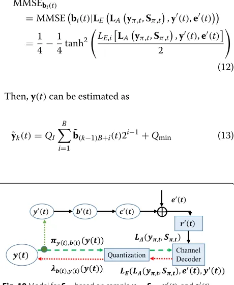
covariance matrixSλ,t. We can simplify the procedure of the message exchanging by substitutingπy(t),b(t)(y(t))and λb(t),y(t)(y(t))withSπ,tandSλ,t, respectively, as shown in Fig. 9. Below, we explain how the averagingSλ,t, i.e.,S¯λ,t, corresponding toSπ,tcan be computed by using iterative decoding.

4.0.4 Quantizing the message between channel decoder

and state estimator

The relationships among yπ,t, Sπ,t, y(t), and channel noise are shown in Fig. 10, wherey(t) is one realization ofπy(t),b(t)(y(t)). Then,y(t)is quantized, modulated, and transmitted over the wireless channel. We denote the cor-responding quantized vector, modulated vector, channel noise vector, and received vector asb(t),c(t),e(t)and

r(t), respectively.

The physical meaning of πy(t),b(t)(y(t)) is the PDF of

y(t). Next, we can useπy(t),b(t)(y(t))as the priori informa-tion to estimate each bit ofb(t)based on its quantization

scheme (the quantization scheme used for convertingy(t)

tob(t)), i.e.,LA(yπ,t,Sπ,t). Note thatLA(yπ,t,Sπ,t)is deter-mined by the PDF, i.e.,πy(t),b(t)(y(t)), and also the quan-tization scheme. Thus,LA(yπ,t,Sπ,t)is aKB-dimensional vector and itsith element can be calculated as

LA,i

yπ,t,Sπ,t

=logP

bi(t)=1|y(t)∈N

yt,yπ,t,Sπ,t

Pbi(t)=0|y(t)∈N

yt,yπ,t,Sπ,t

(9)

The inputs for the channel decoder are LA(yπ,t,Sπ,t) andr(t)shown in Fig. 10. The feedback from the chan-nel decoder to the state estimator is the extrinsic LLR, which is denoted as LE(LA(yπ,t,Sπ,t),y(t), e(t)). It is a

KB-dimension vector and itsith element equals to

LE,i

LA

yπ,t,Sπ,t

,y(t),e(t)

=logP

bi(t)=1|LA

yπ,t,Sπ,t

,r(t) Pbi(t)=0|LA

yπ,t,Sπ,t

,r(t)

(10)

Fig. 9Information exchange between channel decoder and state

where˜si(t)is the estimated-modulated bit and the MMSE in estimating bi(t) from LE(LA(yπ,t,Sπ,t), y(t),e(t)) is

QI is the quantization interval, which is given asQI = Qmax−Qmin

2B₋₁ . Note that when i = j, E{[b˜(k−1)B+i(t) −

b₍k−1)B+i(t)] [b˜(k−1)B+j(t)−b(k−1)B+j(t)]} = 0, which is obtained based on the independence of channel noise and required for the derivation of (14).

Then, for a given πy(t),b(t)(y(t)), which has PDF as N(yt,yπ,t,Sπ,t), a realization y(t), and a channel noise

e(t), the feedback from the channel decoder to the node

y(t) is λb(t),y(t)(y(t)), corresponding to N(yt,yλ,t,Sλ,t), whose mean and covariance matrix are given as

yλ,t= based on one realization,y(t), which is obtained from the PDF ofπy(t),b(t)(y(t)).

4.0.5 Approximation for the message passing between

state estimator and channel decoder

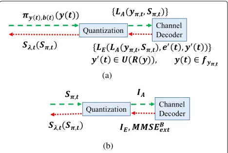
As shown in Fig. 11 (a), for a given πy(t),b(t)(y(t)), the extrinsic information transferred from the channel decoder to the nodey(t)can be computed as require the averaging over a sufficient number of realiza-tions (i.e., large enough to show the probability distribu-tion based on a fixedyπ,t) ofy(t)and the averaging over all possible yπ,t based on its PDF fy_π,t to be computed sequentially, i.e., Forward ProcessandBackward Process

Fig. 11Framework forS_λ,taveraging overy(t)ande(t)

its children, and the Backward Process generally refers to the message passing from a node to its parents. This arises because yπ,t not only impacts priori information

LA(yπ,t,Sπ,t)but also defines the set of codewords which are generated by quantizingy(t).

However, the computation as discussed above prohibits the independent evaluation of the message passing for Forward Process and Backward Process. Thus, to bypass this difficulty, we make the following approximations for the computation ofSλ,t(Sπ,t), so that the Forward Process and Backward Process can be considered separately:

Sλ,t(Sπ,t)=Eyπ,t

First, we approximate the PDF of the realizationsy(t)as a uniform distribution instead ofN(yt,yπ,t,Sπ,t), and we denote the uniform distribution asU(R(y)), whereR(y)is the range ofy(t). Given this approximation, the integra-tion ofy(t)overU(R(y))is equivalent to the integration of all codewords with an equal probability, and hence, the realizationy(t) can be viewed as being independent of πy(t),b(t)(y(t)). Next, as shown in the final step of (18), the averaging overyπ,t can be changed to the averaging overLA(yπ,t,Sπ,t). This exists becauseyπ,t impacts only priori informationLA(yπ,t,Sπ,t)and the setLA(yπ,t,Sπ,t) includes all information fromyπ,t. The framework equiv-alent to (18) is shown in Fig. 12 (a), which is denoted as approximate framework 1, and the computation of

Sλ,t(Sπ,t)in (18) can be divided into the following three steps:

1. Compute the PDF ofLA(yπ,t,Sπ,t)andfyπ,t.

2. Compute the extrinsic information from the channel decoder, i.e., the PDF ofLE(LA(yπ,t,Sπ,t),y(t),e(t)).

3. ComputeSλ,t(Sπ,t)from the extrinsic information

LE(LA(yπ,t,Sπ,t),y(t),e(t)).

Second, we can approximate the PDF of both

LA(yπ,t,Sπ,t) and LE(LA(yπ,t,Sπ,t), y(t), e(t)) as the

Gaussian distributions with zero means. Next, only the covariance matrixes need to be passed through the decoding process. Note thatLE(LA(yπ,t,Sπ,t),y(t),e(t)) for different bits might have a huge difference. This Gaus-sian approximation requires a good interleaver which can evenly distribute LE(LA(yπ,t,Sπ,t),y(t),e(t)). Further-more, if we represent the LLRs by mutual information or MMSE [7] as shown in Fig. 12(b), Sλ,t(Sπ,t) can be computed in the following three steps:

1. Compute the mutual informationIAbased on the

PDF ofLA(yπ,t,Sπ,t)corresponding toSπ,tandfy_π,t. 2. Compute the extrinsic information from the channel

decoder, i.e., mutual informationIEor MMSEBext

based on the PDF ofLE(LA(yπ,t,Sπ,t),y(t)),e(t)).

3. ComputeSλ,t(Sπ,t)from the extrinsic information of

the channel decoderIEor MMSEBext.

5 The MSE transfer chart for channel decoding and state estimation

In this section, we show how to obtain the MSE transfer chart for evaluating BP-based sequential channel decod-ing and state estimation as shown in Fig. 7(b) and BP-based iterative channel decoding and state estimation as shown in Fig. 8(a).

(a)

(b)

Fig. 12Approximate framework forS_λ,taveraging overy(t),e(t)

5.1 The MSE transfer chart for sequential channel decoding and state estimation

The corresponding model to Fig. 7(b) for the MSE trans-fer chart of the sequential message passing is illustrated in Fig. 13 (a). The MSE transfer chart for BP-based sequen-tial channel decoding and state estimation shows the curves between MMSES_ap versus MMSES_ext. As shown in Fig. 13 (a), MMSES_apis used to approximateSπ,t(starting from nodey(t)), i.e.,

Sπ,t=MMSESapIK (19)

and the PDFyπ,t, i.e.,fy_π,t, is assumed to keep the same in all time slots and all iterations. Similarly, MMSES_ext repre-sents the averagingSπ,t+1corresponding toSπ,tandyπ,t with the PDF offyπ,t.

Compared with the model shown in Fig. 7 (b), the MSE transfer chart has two differences. First, the starting node for the message passing is changed fromx(t−1)toy(t). The reason for this changing is to keep alignment with the structure of the MSE transfer chart for BP-based iterative channel decoding and state estimation. Note that since there is no extra information added from nodex(t−1)to

y(t),x(t−1)andy(t)provide the same amount of infor-mation for channel decoding in the context of inforinfor-mation theory. From this point, these two models are equiva-lent. The second modification is that the scalar measures, to draw the MSE transfer chart MMSES_ap and MMSES_ext, rather than the matrix measures are used to evaluate the performance of the sequential message passing.

The value of MMSES_extcan be obtained by applying the results in Table 1, and the message passing flow is shown as a matrix, MMSES_extis calculated by solving the following equation:

IA(MMSESextIK)=IA(Sπ,t+1) (20) where we first obtain the priori informationIAfor each

ith diagonal variance ofSπ,t+1, wherei ∈ {1, ..,K}. Next, to achieve (20), we compute the average value of all the variances, as MMSES_ext. An example of the calculation will be illustrated Section 6.1 in Fig. 15. The physical meaning of (20) is that MMSES_extis the value such that MMSES_extIK can provide the same amount of priori information for the channel decoder asSπ,t+1.

5.2 The MSE transfer chart for BP-based iterative channel decoding and state estimation

In this section, we illustrate how the MSE transfer chart is modeled in order to evaluate the BP-based iterative chan-nel decoding and state estimation as shown in Fig. 8 (a). The corresponding model for the MSE transfer chart is shown in Fig. 13(b), and it includes two flows of the mes-sage passing: one fromy(t)toy(t+1)in Fig. 14(a) and the same in all time slots and all iterations and is denoted byfyπ. MMSEtextrepresents the averageSπ,t+1

(a) (b)

Fig. 14Message passing over two time slots.aTime slot t to t+1.bTime slot t+1 to t

and the PDF ofyπ,t+1isfyπ.

MMSEt_ext+1represents the averagingSπ,t

corresponding toSπ,t=MMSEapt+1IKandyπ,t+1

with the PDF,fy_π.

Then, we obtain two curves: one curve with MMSEt_ap versus MMSEt_ext for the flow from y(t) to y(t+1); the

We consider an electric generator dynamic system for ver-ification. Each dimension of the observationy(t)is quan-tized with 14 bits, and the dynamic range for quantization is [−432, 432]. A 1₂-rate recursive systemic convolution (RSC) code is used as the channel encoding scheme, and the code generator is set asg=[ 1, 1, 1; 1, 0, 1].

The PDF ofyπ,t, i.e., fy_π, is Gaussian with zero mean, and the covariance matrix of yπ,t is obtained from the stationary distribution ofy(t), namely

fy_π =N(y,0,y_π) (23)

whereyπ from the dynamic system is

yπ =

6.1 Message passing between state estimator and channel decoder

In this section, we show the performance results of the proposed channel decoding and state estimation algo-rithm, especially the message passing between the state estimator and channel decoder. In addition, we illustrate how much gain can be obtained by using the redundancy of system dynamics to assist channel decoding. To achieve above, the approximate framework 2 shown in Fig. 12 (b) is considered, but different from that we setSπ,tandSλ,t as MMSEY_apIK and MMSEYextIK.

Figure 15 demonstrates the priori mutual informationIA provided by seven different MMSEY_ap. The curve labeled withDi, corresponding tofyπ,i, complies to a zero-mean Gaussian distribution with variance as ith diagonal ele-ment ofyπ. The curve labeled withmean, corresponding

to fyπ, is a zero-mean Gaussian distribution with the

covariance matrix as yπ. To calculate IA for all eight curves, the curveIA of curve mean is computed as the average of the other IA labeled with D1,· · ·,D7. When MMSEY_apequals to 1.0e−1, 1.1, 1.0e+1, 1.0e+2,IAequals to 0.55, 0, 4, 0.25, 0.15, respectively, and when MMSEY_ap equals to 1.0e+5, the prediction ofy(t)cannot provide any priori information for the channel decoder sinceIAequals to 0. Note that althoughIA can be as high as 0.8 when MMSEY_apequals to 1.0e−3, it is not achievable as the min-imum value of MMSEY_ap is limited by covariance matrix of state dynamics and system observation noise, i.e., nandw.

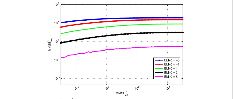
Figure 16 illustrates the relationship between MMSEY_ap and MMSEY_ext. As shown in Fig. 15, the prediction ofy(t)

with MMSES_ap=1.0e+5 does not provide any priori infor-mation for b(t). Therefore, when MMSEt_ap=1.0e+5, the corresponding MMSEt_extis contributed by neither priori informationx(t−1)nor the extrinsic information from the channel decoder at time slott. The gain of MMSEt_extfrom MMSES_apcan be obtained by comparing it with the value of MMSEt_extcorresponding to MMSES_ap=1.0e+5. Follow-ing this flow, the gains of MMSEY_extwith different MMSEY_ap and Eb

Fig. 15Priori mutual information forb₍t₎fromy₍t₎with different MMSEY

ap

6.2 Performance analysis for sequential channel decoding and state estimation

In this section, we show how to use the proposed MSE transfer chart to evaluate the performance of BP-based sequential channel decoding and state estimation over multiple time slots under different channel conditions, where the different channel conditions are modeled by different Eb

N0. Figure 18 shows the relationship between MMSES_ap and MMSES_ext with different Eb

N0. In this figure, we have the following observations:

1. When MMSES_apis less than 1, the corresponding MMSES_extfor all Eb

N0 are equal. Note that MMSE S apis

used to model the amount of priori information from x(t−1). Therefore, the smaller MMSES_apis, the higher amount of priori information attained from x(t−1)is. Although the extrinsic information from the channel decoder at time slott can also contribute to the prediction ofy(t+1), with small MMSES_ap, the priori information fromx(t−1)is dominant in the prediction ofy(t+1). Therefore, the difference of gains from channel decoder with different Eb

N0 is not seen in MMSES_ext.

2. With a large MMSES_ap, the higher Eb

N0 is, the higher MMSES_extis. With the increasing of MMSES_ap, x(t−1)provides less amount of priori information

Fig. 16MMSEY_extwith different MMSEY_apandEb

Fig. 17Gain of MMSEY

extwith different MMSEYapwithENb0

for the predictiony(t), and the extrinsic information from channel decoder becomes dominant in the prediction ofy(t). Then, the channel gains with different Eb

N0 are seen.

3. When MMSES_apis around 1.0e−2, the values MMSES_extare flat. This arises because, based on the information from the time slots priori tot+1, the prediction ofy(t)is not reliable since state dynamics n(t)and the noise of system observationw(t)are not predictable. This leads that the minimum value of MMSES_extis limited by the covariance matrix ofn(t) andw(t), i.e.,nandw, respectively.

Following the same idea of the EXIT chart and the MSE transfer chart for iterative channel decoding, we use the MSE transfer chart to evaluate the performance of BP-based sequential channel decoding and state estima-tion over mutiple time slots. In the MSE transfer chart, we have two curves: one is MMSES,t_ap versus MMSES,t_ext, which is equivalent to the curve for MMSES_ap versus MMSES_ext(MMSES_apand MMSES_extat time slott); the other is MMSES,t_ext+1versus MMSES,t_ap+1, which is equivalent to the flipped curve for MMSES_apversus MMSES_ext(MMSES_ap and MMSES_extat time slott+1).

Fig. 18Relationship between MMSES_extand MMSES_apfor the sequential message passing with different Eb

The MSE transfer chart for Eb

N0 =5 dB is shown in Fig. 19. There is one crossing/convergence point between these two curves, which means that it is not a

success-ful decoding from IA = 0 to IA = 1. The arrows

with black color show the trace of the sequential message passing(starting from MMSES_ap=1.0e−2 at time slot t). We can see that trace moves toward the convergence point at time slot t + 1 and t + 2. The trace shows that even if we have perfect knowledge of y(t) at time slot t, the performance of state estimation degrades toward the crossing point after running a few time slots. The arrows with red color show the other trace (starting from MMSES_ap=1.0e+5), at which there is no priori information from the prediction of y(t). Sim-ilarly, we can see the trace is moving toward the convergence point at time slot t + 1,t + 2,· · ·. Different from the above, this trace shows that even though there is no priori information ofy(t)at time slot

t, the performance of state estimation is improved after running a few time slots, and finally, the gain reaches the convergence point.

Figure 20 illustrates the MSE transfer chart as Eb

N0 =3 dB

with one crossing point at MMSES,t_ap=1.0e−0.15. In the range of [1.0e−0.15, 1.0e+2], the gap between the curve (MMSES,t_ap versus MMSES,t_ext) and the flipped curve (MMSES,t_ext+1 versus MMSES,t_ap+1) is very small. This means that the convergence speed is slow and it takes many time slots to converge to the convergence point when the state estimator has no priori information ofy(t)

at time slott.

Figure 21 shows the MSE transfer chart as Eb

N0 =1 dB

with one crossing point at MMSES,t_ap=1.0e−0.15. Note

that after the crossing point the curve (MMSES,t_ap ver-sus MMSES,t_ext) almost overlaps with the flipped curve (MMSES,t_ext+1 versus MMSES,t_ap+1). This shows two condi-tions when the state estimator has no priori information ofy(t) at time slott: one is that it will gain a high MSE and cannot coverage to the crossing point; the other is that it will take many time slots to converge to the crossing point. Compared with previous two results, for Eb

N0=1 dB, the MSEs of estimatingx(t)andy(t)are much higher than that for Eb

N0 equals to 3 and 5 dB. Similar results go with the case when Eb

N0 = −1 dB.

6.3 Performance analysis for iterative channel decoding and state estimation

In this section, we show how to use the proposed MSE transfer chart to evaluate the performance of BP-based iterative channel decoding and state estimation within two time slots. As we stated, the nodex(t−1)and the nodey(t)

provide the same amount of information in the context of information theory. From this point, the priori informa-tion at the nodey(t), as same as the nodex(t−1), will beπx(t−1),x(t)(x(t−1)) = N(xt−1,xπx,t−1,Pπx,t−1) with

xπx,t−1=0andPπx,t−1=MMSE t−1,x

ap Ik.

With the priori information as an initial input for itera-tive decoding, the gains of MMSEt_ext(based on MMSEt_ap) with different MMSEt_ap−1,x and Eb

N0=5 dB are illustrated in Fig. 22, and from this figure, we have the following observations:

1. With the same MMSEt_ap−1,x, the higher MMSEt_apis, the lower gain of MMSEt_extcan be obtained from MMSEt_ap.

Fig. 19The MSE transfer chart for sequential channel decoding and state estimation:Eb

Fig. 20The MSE transfer chart for sequential channel decoding and state estimationEb

N0=3 dB

2. The higher the MMSEt_ap−1,xis, the higher gain of MMSEt_extcan be obtained from MMSEt_ap. This exists because the prediction ofy(t+1)is contributed by both priori information fromx(t−1)and the extrinsic information from the channel decoder at time slott. When MMSEt_ap−1,xis small, the

information fromx(t−1)is dominant in predicting y(t+1). Although the prediction ofy(t)can increase the amount of extrinsic information from channel decoder at time slott, it cannot contribute much to the gain of MMSEt_extas the priori information from x(t−1)is dominant.

Following the same idea, the gain of MMSEt_ext+1 (based on MMSEt_ap+1) is obtained and shown in Fig. 23. Similar observations as above are obtained:

1. With the same MMSEt_ap−1,x, the higher MMSEt_ap+1is, the lower gain of MMSEt_ext+1can be obtained from MMSEt_ap.

2. The higher the MMSEt_ap−1,xis, the higher gain of MMSEt_ext+1can be obtained from MMSEt_ap+1.

Then, the MSE transfer chart for BP-based iterative channel decoding and state estimation is formed by the

Fig. 21The MSE transfer chart for sequential channel decoding and state estimationEb

Fig. 22Gain of MMSEt

extfrom MMSEtapwith different MMSEtap−1,xandNEb0=5 dB

curve (MMSEt_apversus MMSEt_ext) and the flipped curve (MMSEt_ap+1versus MMSEt_ext+1), and the results with differ-ent MMSEt_ap−1,xand Eb

N0 =5 dB are shown in Fig. 24. In the following, we try to explain our observations based on the case where no priori information are considered.

1. BP-based iterative channel decoding can decrease MMSEt_extand help improve the estimation of x(t+1). The values of the crossing point between the curve (MMSEt_apversus MMSEt_ext) and the flipped curve (MMSEt_ap+1versus MMSEt_ext+1) for MMSEt_apand MMSEt_extare 1.0e+1.33 and 1.0e+1.25, respectively, while the values of MMSEt_apand MMSEt_extwith no priori information are 1.0e+5 and 1.0e+1.43,

respectively. Therefore, the total gain of MMSEt_extfor BP-based iterative channel decoding and state estimation is10∗(1.43−1.25)=1.8 dB.

2. The gain of MMSEt_extwith only three steps is close to the gain of MMSEt_extat the convergence point. The trace of BP-based iterative channel decoding and state estimation with the mentioned three steps is shown by the arrows with blue color in the figure, and the details are listed as below:

1) Fromy(t)toy(t+1): As there is no priori information, the starting point is MMSEt_ap with the value of 1.0e+5, and the

corresponding value of MMSEt_extis 1.0e+1.43.

Fig. 23Gain of MMSEt_ext+1from MMSE_apt+1with different MMSEt_ap−1,xandEb

Fig. 24MSE-based transfer chart for iterative channel decoding and system state estimation with different MMSEt−1,x

ap andNEb0=5 dB

2) Fromy(t+1)toy(t): We have MMSEt_ap+1with the value of 1.0e+1.43, and the corresponding value of MMSEt_ext+1is 1.0e+1.34.

3) Fromy(t)toy(t+1): We have MMSEt_apwith the value of 1.0e+1.34, and the corresponding value of MMSEt_extis 1.0e+1.255. Compared with step (1),10∗(1.43−1.255)=1.75 dB is obtained for MMSEt_extwhile it is 1.8 dB for MMSEt_extfrom convergence point. Thus, the gain loss for BP-based iterative channel decoding and state estimation with these three steps is just1.8−1.75=0.05 dB.

In summary, we can implement BP-based iterative channel decoding and state estimation with above three steps to obtain the gain of MMSEt_ext, which is close to the gain at convergence point.

Note that when MMSEt_ap−1,x equals to 1 or 10, the BP-based iterative channel decoding and state estimation scheme cannot improve the performance of state estima-tion. This is because with a small MMSEt_ap−1,x the priori information fromx(t)is dominant in estimatingy(t+1), which leads that the prediction ofy(t)in channel decoder at time slottis negligible in predictingy(t+1).

Fig. 25MMSEY_totwith different MMSEY_apandEb

Fig. 26Gain of MMSEY_totwith different MMSEY_apandEb

N0

The MSE transfer charts for Eb

N0 =3 and 1 dB have sim-ilar observations as that for Eb

N0 =5 dB, so we will not list the results here.

6.4 Performance analysis for Kalman filtering-based heuristic approach

Similarly, by utilizing the redundancy of system dynam-ics, a Kalman filtering-based heuristic approach is eval-uated in this section. In the Kalman filtering-based heuristic approach, the prediction of y(t) based on Kalman filtering is used as the priori information for

b(t), and instead of using only the extrinsic information of the channel decoder to obtain a soft estimation of

y(t), the total information including both the pri-ori information and the extrinsic information gener-ated by the channel decoder is used to obtain a hard estimation ofy(t).

The corresponding framework used for the Kalman filtering-based heuristic approach is similar to the BP-based channel decoding and state estimation as shown in Fig. 12 (b). The priori information from y(t) is modeled with Sπ,t = MMSEYapIK, and the priori information for b(t) is represented by mutual informa-tion IA. Finally, the total information from the chan-nel decoder for estimating of b(t) is modeled by MMSEB_tot, which means the MMSE of estimating b(t)

based on the total information including both the pri-ori information and the extrinsic information from the channel decoder.

Figure 25 illustrates the relationship between MMSEY_ap and MMSEY_tot. The gains of MMSEY_tot with different MMSEY_ap and Eb

N0 are shown in Fig. 26, which are further improved comparing to Fig. 17.

7 Conclusions

We propose to use the MSE transfer chart to evaluate the performance of BP-based channel decoding and state esti-mation. We focus on two models, the BP-based sequential processing model and the BP-based iterative processing model, for channel decoding and state estimation. The for-mer can be used to evaluate the performance of sequential processing over multiple time slots, and the latter can be used to evaluate the performance of iterative process-ing within two time slots. The numerical results show by utilizing the MSE transfer chart the proposed chan-nel decoding and state estimation algorithm can decrease the MSE and improve performance of channel decoding and state estimation. Specifically, a total 1.75 dB gain can be earned through three-step BP-based iterative chan-nel decoding and state estimation process when no prior information is given.

Acknowledgements

The authors would like to thank the support of National Science Foundation under grants ECCS-1407679, CNS-1525226, CNS-1525418, and CNS-1543830.

Authors’ contributions

HL conceived the Brainbow strategies for this work. JBS and HL supervised the project. SG built the initial constructs and LL validated them, analyzed the data, and wrote the paper. All authors read and approved the final manuscript.

Competing interests

The authors declare that they have no competing interests.

Publisher’s Note

Springer Nature remains neutral with regard to jurisdictional claims in published maps and institutional affiliations.

Author details

1_{Department of Electrical Engineering and Computer Science, the University}

of Tennessee, Knoxville, Knoxville, USA.2Sequans Communications, 1732, Deogyoung Road, 446701 Giheung, Yongin, South Korea.3_{Department of}

and applications in smart grids. (Morgan Kaufmann, Cambridge, 2016) 3. S ten Brink, Convergence of iterative decoding. Electron. Lett.35(10),

806–808 (1999)

4. S Ten Brink, inProceedings of 3rd IEEE/ITG Conference on Source and Channel Coding, Munich, Germany. Iterative decoding trajectories of parallel concatenated codes, (2000), pp. 75–80

5. S Ten Brink, Convergence behavior of iteratively decoded parallel concatenated codes. IEEE Trans. Commun.49(10), 1727–1737 (2001) 6. M El-Hajjar, L Hanzo, Exit charts for system design and analysis. IEEE

Commun. Surveys Tutorials.16(1), 127–153 (2013)

7. K Bhattad, KR Narayanan, An MSE-based transfer chart for analyzing iterative decoding schemes using a Gaussian approximation. IEEE Trans. Inf. Theory.53(1), 22–38 (2007)

8. A Ashikhmin, G Kramer, S ten Brink, Extrinsic information transfer functions: model and erasure channel properties. IEEE Trans. Inf. Theory.

50(11), 2657–2673 (2004)

9. D Guo, S Shamai, Verdú, Mutual information and minimum mean-square error in Gaussian channels. IEEE Trans. Inf. Theory.51(4), 1261–1282 (2005) 10. M Fu, CE de Souza, State estimation for linear discrete-time systems using

quantized measurements. Automatica.45(12), 2937–2945 (2009) 11. S Yüksel, Ba¸s,ar, Stochastic networked control systems. AMC.10, 12 (2013) 12. L Li, H Li, inGlobal Communications Conference (GLOBECOM), 2016 IEEE.

Dynamic state aware source coding for networked control in cyber-physical systems (IEEE, Washington, DC, 2016), pp. 1–6

13. S Yüksel, On stochastic stability of a class of non-Markovian processes and applications in quantization. SIAM J. Control. Optim.55(2), 1241–1260 (2017)

14. N Ramzan, S Wan, E Izquierdo, Joint source-channel coding for wavelet-based scalable video transmission using an adaptive turbo code. EURASIP J. Image Video Process.2007(1), 1–12 (2007)

15. V Kostina, Verdú, Lossy joint source-channel coding in the finite blocklength regime. IEEE Trans. Inf. Theory.59(5), 2545–2575 (2013) 16. H Wu, L Wang, S Hong, J He, Performance of joint source-channel coding

based on protograph LDPC codes over Rayleigh fading channels. IEEE Commun. Lett.18(4), 652–655 (2014)

17. X He, X Zhou, P Komulainen, M Juntti, T Matsumoto, A lower bound analysis of hamming distortion for a binary ceo problem with joint source-channel coding. IEEE Trans. Commun.64(1), 343–353 (2016) 18. Y Wang, M Qin, KR Narayanan, A Jiang, Z Bandic, inGlobal

Communications Conference (GLOBECOM), 2016 IEEE. Joint Source-Channel Decoding of Polar Codes for Language-Based Sources (IEEE, Washington, DC, 2016), pp. 1–6

19. V Kostina, Y Polyanskiy, S Verd, Joint source-channel coding with feedback. IEEE Trans. Inf. Theory.63(6), 3502–3515 (2017) 20. L Yin, J Lu, Y Wu, inCommunication Systems, 2002. ICCS 2002. The 8th

International Conference On. LDPC-based joint source-channel coding scheme for multimedia communications, vol. 1 (IEEE, Singapore, 2002), pp. 337–341

21. J Garcia-Frias, W Zhong, LDPC codes for compression of multi-terminal sources with hidden Markov correlation. IEEE Commun. Lett.7(3), 115–117 (2003)

22. W Zhong, Y Zhao, J Garcia-Frias, inConference Record of the Thirty-Seventh Asilomar Conference on Signals, Systems and Computers. Turbo-like codes for distributed joint source-channel coding of correlated senders in multiple access channels (IEEE, Pacific Grove, 2003), pp. 840–844 23. Z Mei, L Wu, Joint source-channel decoding of Huffman codes with LDPC

codes. J Electron (China).23(6), 806–809 (2006)

24. X Pan, A Cuhadar, AH Banihashemi, Combined source and channel coding with JPEG2000 and rate-compatible low-density parity-check codes. IEEE Trans. Signal Process.54(3), 1160–1164 (2006)

nonbinary sources using punctured turbo codes. IEEE Trans. Commun.

53(3), 385–390 (2005)

30. R Gallager, Low-density parity-check codes. IRE Trans. Informa. Theory.

8(1), 21–28 (1962)