R E S E A R C H
Open Access
Conservation laws, analytical solutions and
stability analysis for the time-fractional
Schamel–Zakharov–Kuznetsov–Burgers
equation
O.H. EL-Kalaawy
1*, S.M. Moawad
1, M.M. Tharwat
1and Rasha B. Al-Denari
1*Correspondence:
1Department of Mathematics and
Computer Science, Faculty of Science, Beni-Suef University, Beni-Suef, Egypt
Abstract
In this paper, we consider the (3 + 1)-dimensional time-fractional
Schamel–Zakharov–Kuznetsov–Burgers (SZKB) equation. With the help of the Riemann–Liouville derivatives, the Lie point symmetries of the (3 + 1)-dimensional time-fractional SZKB equation are derived. By applying the Lie point symmetry method as well as Erdélyi–Kober fractional operator, we get the similarity reductions of the time-fractional SZKB equation. Conservation laws of the time-fractional SZKB are constructed. Moreover, we obtain its power series solutions with the convergence analysis. In addition, the analytical solution is obtained by modified trial equation method. Finally, stability is analyzed graphically in different planes.
Keywords: Lie point symmetries; Conservation laws; Time-fractional
Schamel–Zakharov–Kuznetsov–Burgers equation; Riemann–Liouville derivatives; Similarity reduction; Explicit power series; Modified trial equation
1 Introduction
Partial differential equations (PDEs) are frequently used to describe most of the phe-nomena that arise in engineering fields, mathematical physics, plasma physics, solid state physics, quantum mechanics, fluid mechanics, ecology, optical fibers, biology, chemical kinematics, geochemistry, meteorology, electricity and so on. Therefore, investigating an-alytical solutions (traveling wave solutions or soliton solutions) is very interesting. As a result, many new techniques have been successfully proposed, developed and extended by groups of researchers to find exact or analytical solutions for PDEs, such as the (G/G )-expansion method [1–3], the Kudryashov method [4,5], the functional variable method [5,6], the first integral method [7], theexp(–φ(ξ))-expansion method [8], the sine–cosine function method and Bernoulli’s equation approach [5,9], the trial solution method [5, 10], Hirota’s bilinear method [3] etc.
Fractional calculus was developed as one of the best tools for studying various models in each discipline [11,12]. Using fractional models to describe the special characteristic phenomenon of fractional order, it can well reveal the essence of the nature of phenom-ena and their behavior. Fractional calculus is a generalization of integer calculus, integer
calculus is a special case of fractional calculus. It has universal significance to study the fractional calculus system. Compared with the integer order model in describing the ac-tual physical process, the physical meaning of the fractional order model is clearer and the expression is more concise.
On the other hand, in recent years, fractional ordinary differential equations (FODEs) and fractional partial differential equations (FPDEs) have been widely used to describe many various physical effects and many complex nonlinear phenomena. This is due to their accurate description of nonlinear phenomena in fluid mechanics, viscoelasticity, electrical chemistry, quantum biology, physics, engineering mechanics [13–19] and other scientific fields. So the study of FODEs and FPDEs has attracted much attention. In other words, by using the theory of derivatives and integrals of fractional order, many physical phenomena can be accurately modeled.
The exact solutions of most of the FPDEs cannot be found easily, so analytical and nu-merical methods [20,21] must be used. The solutions of the FPDEs are investigated by many authors using powerful analytical methods. Several numerical methods such as the homotopy perturbation method [22,23], the Adomian decomposition method [24], the variational iteration method [25], the differential transform method [26], the fractional Riccati expansion method [27], the fractional sub-equation method [28–34] have been suggested for solving FDEs. However, solutions obtained through all these methods are of a local nature and it is important to explore other techniques in order to find exact analytical solutions of FDEs.
Lie point symmetry plays a very important role in various fields of science, especially in integrable systems where infinitely many symmetries exist. So Lie symmetry analy-sis is considered to be one of the efficient approaches for obtaining analytical solutions of nonlinear partial differential equations (NLPDEs). A large number of studies are de-voted to the theory of Lie point symmetry and their applications to DEs. The symmetry analysis of FDEs and the fractional derivatives are proposed by Gazizov and his collab-orators [35]. They proposed a prolongation formula for two basic fractional derivatives: Riemann–Liouville and Caputo. This method has been used to study many of the FDEs [36–38]. Furthermore Lie point symmetry is used to construct conservation laws which play an important role in the study of nonlinear physical phenomena [12]. Conservation laws are a mathematical formulation which statement that the total amount of a certain physical quantity stays the same during the evolution of a physical system [12]. Conserva-tion laws are also used in the development of numerical methods to establish the existence and uniqueness of solution. There are many methods of constructing conservation laws for differential equations (DEs) [39–45]. The well-known Noether theorem [46] establishes a connection between Lie point symmetries and conservation laws of DEs, provided that the equations are Euler–Lagrange equations. Ibragimov [47] suggested a new conservation law theorem. In [39], conservation laws for time-fractional sub-diffusion and diffusion-wave equations were obtained based on the new conservation laws theorem [47]. Also there are researches that discussed conservation laws for time FPDEs [12,48,49].
In this work, we focus on the time-fractional SZKB equation of the form
∂αu
∂tα +a
√
uux+buxxx+c(uxyy+uxzz) +duxx= 0, (1.1)
where∂α
t is the fractional derivative of orderα, with 0 <α< 1 andu(x,y,z,t) is the
equation, which describes the nonlinear plasma-dust ion acoustic waves DIAWs in a mag-netized dusty plasma and it is derived using the standard reductive perturbation technique in small amplitude. The coefficients of dispersionb, non-linearitya, mixed derivativecand dissipationdare given in [50,51].Note that Sahoo and Ray[52]have studied the(3 + 1) -dimensional time-fractional mKdV-ZK equation without the Schamel and Burgers terms. The main purpose of this paper is to obtain the Lie point symmetries, conservation laws and analytical solutions of the time-fractional SZKB equation.
The paper is organized as follows: The introduction is presented in Sect.1. In Sect.2, some definitions and description of Lie symmetry analysis for fractional partial differential equations (FPDEs) are briefly presented. Lie point symmetries and similarity reduction of the Eq. (1.1) are obtained In Sect.3. In Sect.4, the conservation laws of the Eq. (1.1) are obtained. In Sect. 5, which is based on the power series, the analytical solution of the Eq. (1.1) is constructed with convergence analysis. We construct the analytical solution of Eq. (1.1) by using a modified trial equation method In Sect.6. Finally, the discussions and conclusions of this paper are presented in Sect.7.
2 Preliminaries
Here in this section, we focus on some of the concepts that revolve around the subject of our article
Definition 1 Letα> 0. The operatorIαdefined by
Iαf(t) = 1
Γ(α)
t
0
(t–s)α–1f(s)ds, (2.1)
is called the Riemann–Liouville (R-L) fractional integral operator of order α, andΓ(·) denotes the gamma function.
Definition 2 Letα> 0. The operatorDα
t defined by
Dα
tf(t) = ⎧ ⎨ ⎩
1
Γ(n–α) dn dtn
t 0(t–s)n–
α–1f(s)ds ifn– 1 <α<n,n∈N,
dnf(t)
dtn ifα=n,n∈N,
(2.2)
is called the R-L fractional partial derivative [16,53–56].
2.1 Description of Lie point symmetries
Let us consider the symmetry analysis for a FPDE of the form
Dα
tu(x,y,z,t) =G(x,y,z,t,u,ux,ut,uy,uz,uxx,uxy, . . .), 0 <α< 1. (2.3)
Now, let Eq. (2.3) be invariant under the following one-parameter Lie group of point trans-formations acting on both the dependent and the independent variables:
¯
x=x+εξ(x,y,z,t) +Oε2,
¯
y=y+εζ(x,y,z,t) +Oε2,
¯
¯
t=t+ετ(x,y,z,t) +Oε2,
¯
u=u+εη(x,y,z,t) +Oε2,
Dα¯tu¯=Dαtu+εη0α(x,y,z,t) +O
ε2, (2.4)
∂u¯
∂x¯ =
∂u
∂x+εη
x(x,y,z,t) +Oε2,
∂2u¯
∂x¯2 =
∂2u
∂x2 +εη
xx(x,y,z,t) +Oε2,
∂3u¯
∂x¯3 =
∂3u
∂x3 +εη
xxx(x,y,z,t) +Oε2,
∂3u¯
∂x¯∂y¯2 =
∂3u
∂x∂y2 +εη
xyy(x,y,z,t) +Oε2,
∂3u¯
∂x¯∂z¯2 =
∂3u
∂x∂z2+εη
xzz(x,y,z,t) +Oε2,
whereε1 is the Lie group parameter andξ,ζ,ν,τ,ηare the infinitesimals of the trans-formations for dependent and independent variables, respectively. The explicit expres-sions ofηx,ηxx,ηxxx,ηxyy,ηxzzare given by
ηx=Dx(η) –uxDx(ξ) –uyDx(ζ) –uzDx(ν) –utDx(τ),
ηxx=Dx
ηx–uxxDx(ξ) –uxyDx(ζ) –uxzDx(ν) –uxtDx(τ),
ηxxx=Dx
ηxx–uxxxDx(ξ) –uxxyDx(ζ) –uxxzDx(ν) –uxxtDx(τ),
ηxyy=Dx
ηyy–uxxyDx(ξ) –uxyyDx(ζ) –uxyzDx(ν) –uxytDx(τ),
ηxzz=Dx
ηzz–uxxzDx(ξ) –uxyzDx(ζ) –uxzzDx(ν) –uxztDx(τ),
(2.5)
whereDx,Dy,Dz, andDtare the total derivatives with respect tox,y,z, andt, respectively,
that are defined forx1=x,x2=y,x3=zas
Dxj=
∂ ∂xj+uj
∂ ∂u+ujk
∂ ∂uk
+· · ·, j,k= 1, 2, 3, . . . ,
whereuj=∂∂xuj,ujk= ∂
2u
∂xj∂xk and so on.
The corresponding Lie algebra of symmetries consists of a set of vector fields of the form
V=ξ ∂ ∂x+ζ
∂ ∂y+ν
∂ ∂z+τ
∂ ∂t+η
∂ ∂u.
The invariance condition of Eq. (2.3) under the infinitesimal transformations is given as
Pr(n)V() =0= 0, n= 1, 2, 3, . . . ,
where
Also, the invariance condition gives
τ(x,y,z,t,u)|t=0= 0. (2.6)
Theαth extended infinitesimal related to RL fractional time derivative with Eq. (2.6) can be represented as follows:
η0α=Dα
t is the total fractional derivative operator and by using the generalized Leibnitz
rule
By applying the Leibnitz rule, Eq. (2.7) becomes
η0α=Dαt(η) –αDαt(τ)∂
Now the chain rule for the compound function is defined as follows:
dnφ(h(t))
By applying this rule and the generalized Leibnitz rule withf(t) = 1, we have
Dαt(η) =∂
Therefore, Eq. (2.8) yields
Definition 3 The functionu=θ(x,y,z,t) is an invariant solution of Eq. (2.3) associated with the vector fieldW, such that
1. u=θ(x,y,z,t)is an invariant surface of Eq. (2.3), this means
3 Lie point symmetries and similarity reduction for Eq. (1.1)
In this section, we implemented Lie group method for Eq. (1.1) and then, used these sym-metries to reduce Eq. (1.1) to be a FODE as shown in the next two subsections
3.1 Lie point symmetries for Eq. (1.1)
Let us consider Eq. (1.1) as an invariant under Eq. (2.4), we get
∂αu¯ in Eq. (3.1), we get the invariant equation
η0α+a√uηx+ a
2√uηux+bη
xxx+cηxyy+ηxzz+dηxx= 0, (3.2)
By substituting Eq. (2.5) and Eq. (2.9) into Eq. (3.2), we acquire
+ (2ηxuy+ 2ηuuyux–ζxyy–ζuyyux)uy+ (ηu– 2ζy–ξx–ζuux)uxyy
+ 2(ηuu– 2ζuy)uyuxy+ (ηxu+ηuuux– 2ζxy– 2ζuyux)uyy– 3ζuuu2yuxy
+ (3ηuux+ηuuuux– 2ζxuy– 2ζuuyux)uy2– 3ζuuxyuyy– (ζuux+ζuuuux)u3y
– 3ζuuyuxyy– 3(ζxu+ζuuux)uyuyy– (2ξy+ 2ξuuy+ξx+ξuux)uxxy
– 2(ξuyux+ξxuuy+ξuuuxuy+ξuuxy)uxy– (2νy+ 2νuuy+νx+νuux)uxyz
– 2(νuyux+νxuuy+νuuuxuy+νuuxy)uzy(2τy+ 2τuuy+τx+τuux)uxyt
– 2(τuyux+τxuuy+τuuuxuy+τuuxy)uyt–
ξyyux+ 2ξuyuy+ξuuu2y+ξuuyy
uxx
–νyy+ 2νuyuy+νuuu2y+νuuyy
uxz–
τyy+ 2τuyuy+τuuu2y+τuuyy
uxt
–ξxyy+ξuyyux+ 2ξxyuuy+ 2ξuuyuxuy+ 2ξuyuxy+ξxuuu2y+ξuuuuxu2y+ 2ξuuuxuxy
+ξxuuyy+ξxuuxuyy+ξuuxyy
ux–
νxyy+νuyyux+ 2νxyuuy+ 2νuuyuxuy+ 2νuyuxy
+νxuuu2y+νuuuuxu2y+ 2νuuuxuxy+νxuuyy+νxuuxuyy+νuuxyy
uz
–τxyy+τuyyux+ 2τxyuuy+ 2τuuyuxuy+ 2τuyuxy+τxuuu2y+τuuuuxu2y+ 2τuuuxuxy
+τxuuyy+τxuuxuyy+τuuxyy
ut+ηxzz+ (ηuzz–ξxzz)ux+ (2ηuy–ζyy– 2ξxy)uxz
+ (2ηxuz+ 2ηuuzux–νxzz–νuzzux)uz+ (ηu– 2νz–ξx–νuux)uxzz
+ 2(ηuu– 2νuz)uzuxz+ (ηxu+ηuuux– 2νxz– 2νuzux)uzz– 3νuuu2zuxz
+ (3ηuux+ηuuuux– 2νxuz– 2νuuzux)u2z– 3νuuxzuzz– (νuux+νuuuux)u3z– 3νuuzuxzz
– 3(νxu+νuuux)uzuzz– (2ξz+ 2ξuuz+ξx+ξuux)uxxz
– 2(ξuzux+ξxuuz+ξuuuxuz+ξuuxz)uxz– (2ζz+ 2ζuuz+ζx+ζuux)uxyz
– 2(ζuzux+ζxuuz+ζuuuxuz+ζuuxz)uzy– (2τz+ 2τuuz+τx+τuux)uxzt
– 2(τuzux+τxuuz+τuuuxuz+τuuxz)uzt–
ξzzux+ 2ξuzuz+ξuuu2z+ξuuzz
uxx
–ζzz+ 2ζuzuy+ζuuu2z+ζuuzz
uxy–
τzz+ 2τuzuy+τuuu2z+τuuzz
uxt
–ξxzz+ξuzzux+ 2ξxzuuz+ 2ξuuzuxuz+ 2ξuzuxz+ξxuuu2z+ξuuuuxu2z+ 2ξuuuxuxz
+ξxuuzz+ξxuuxuzz+ξuuxzz
ux–
ζxzz+ζuzzux+ 2ζxzuuz+ 2ζuuzuxuz+ 2ζuzuxz
+ζxuuu2z+ζuuuuxu2z+ 2ζuuuxuxz+ζxuuzz+ζxuuxuzz+ζuuxzz
uy
–τxzz+τuzzux+ 2τxzuuz+ 2τuuzuxuz+ 2τuzuxz+τxuuu2z
+τuuuuxu2z+ 2τuuuxuxz+τxuuzz+τxuuxuzz+τuuxzz
ut)
+dηxx+ (2ηxu–ξxx)ux+ (ηu– 2ξx)uxx+ (ηuu– 2ξxu)u2x–ξuuu3x– 3ξuuxuxx
– 2(ζx+ζuux)uxy– 2(νx+νuux)uxz– 2(τx+τuux)uxt
–ζxx+ 2ζxuux+ζuuu2x+ζuuxx
uy–
νxx+ 2νxuux+νuuu2x+νuuxx
uz
–τxx+ 2τxuux+τuuu2x+τuuxx
ut
now, for Eq. (3.3) by making the whole powers of derivatives ofuto zero, we get the fol-lowing system of equations:
α
n
∂αη
u
∂tα –
α
n+ 1
Dn+1t (τ) = 0, n= 1, 2, 3, . . . ,
a 2√uη+a
√
u(ηu–ξx) +b(3ηxxu–ξxxx) +c(ηyyu–ξxyy+ηzzu–ξxzz) +d(2ξxu–ξxx) = 0,
a√uηx+bηxxx+c(ηxyy+ηxzz) +dηxx+μ= 0,
τu=ξu=νu=τx=ζu=νu= 0,
τuu=ξuu=νuu=ζuu=νuu= 0,
Dnt(ξ) = 0, n= 1, 2, 3, . . . ,
ηu–αDt(τ) = 0,
ηu– 2ζy–ξx= 0,
ηu– 3ξx= 0,
ηu– 2νz–ξx= 0.
On solving the previous system of equations, we get the following infinitesimals:
ξ=c1x+c2, τ=
3
αc1t+c3, ζ =c1y+c4, ν=c1z+c5, η= –4c1u, (3.4)
whereci,i= 1, 2, 3, 4, 5 are arbitrary constants. So, the associated vector fields are given by
V1=
∂
∂x, V2=
∂
∂t, V3=
∂
∂y, V4=
∂ ∂z,
V5=x
∂ ∂x+y
∂ ∂y+z
∂ ∂z+
3
αt ∂ ∂t– 4u
∂ ∂u,
(3.5)
and then, all of the infinitesimal generators of Eq. (1.1) can be expressed as follows:
V=c1V1+c2V2+c3V3+c4V4+c5V5.
3.2 The similarity reduction for Eq. (1.1)
In order to reduce Eq. (1.1) to become a FODE, we used the infinitesimal generatorV5
defined in Eq. (3.5) to form the following characteristic equation:
dx x =
dy y =
dz z =
dt
3
αt = du
–4u.
Solving the above equation yields the following similarity function:
u=t–43αf(ξ), ξ= (x+y+z)t–α3. (3.6)
Theorem 1 The transformation equation(3.6)reduces the time-fractional SZKB Eq. (1.1)
to the following nonlinear FODE:
is the EK fractional integral operator.
Proof Letn– 1 <α< 1,n= 1, 2, 3, . . . , we obtain the similarity transformation based on Riemann–Liouville fractional derivatives as follows:
∂αu
by using the definition of EK fractional differential operator, then Eq. (3.11) becomes
and thus repeating we have
On using the definition of the EK fractional differential operator Eq. (3.9), we get
∂n
By substituting Eq. (3.13) into Eq. (3.12), we have
∂αu
Thus, Eq. (3.13) can be reduced into a fractional ordinary differential equation
The proof of the theorem is completed.
4 Conservation laws for Eq. (1.1)
In this section, the conservation laws of the time-fractional SZKB equation (1.1) are de-rived, based on the formal lagrangian and Lie point symmetries as described in the fol-lowing explanation:
servation theorem due to Ibragimov [47], the formal Lagrangian for Eq. (1.1) can be given by grangian, we get an action integral as follows:
The Euler–Lagrange operator is defined as
t)∗denotes to the adjoint operator ofDαt, and the adjoint equation to the
non-linear by means of the Euler–Lagrange equation given by
δL
δu= 0.
The adjoint operator (Dα
t)∗for R-L is defined by
Dαt∗= (–1)nITn–αDnt≡CtDαT,
whereIn–α
T is the right-sided operator of fractional integration of ordern–αthat is defined
by
Considering the case of one dependent variableu(x,y,z,t) with four independent variables x,y,z,t, we get
and the Lie characteristic function is defined by
W=η–τut–ξux–ζuy–νuz, and then
W1= –ux, W2= –ut, W3= –uy, Wt= –uz.
(4.3)
For the R-L time-fractional derivative, the density componentCt of conservation law is
and the other (flux) components are defined as
Now by using Eq. (4.3) with the help of Eqs. (4.4) and (4.5), we obtain the components of the conservation laws for the time-fractional SZKB equation as follows.
C3y=ω
Dαtu+a√uux+
c
3(uyxy+uyyx+uzxz+uzzx) +duxx
–c
3uy[ωxy+ωyx] + c
3(uxyωy+uyyωx) – c
3ω(uxyy+uyxy),
C3z= –c
3uy[ωxz+ωzx] + c
3(uxyωz+uyzωx) – c
3ω(uxzy+uzxy).
Case 4:W4= –uzwhereξx= 0,ξt= 0,ξy= 0,ξz= 0 andη= 0 we obtain the following
conserved vectors:
C4t=ω0Dαt–1(–uz)
∂L
∂0Dαtu
–J
–uz,Dnt
∂L
∂0Dαtu
= –ωDαt(uz) –uzDαt(ω),
C4x= –uz
aω√u–dωx+bωxx+
c
3(ωyy+ωzz)
–uxy[dωx–bωx]
+c
3(uyyωy+uyzωz) –bωuxxy– c
3ω(uyyy+uzzy),
C4y=ω
Dαtu+a√uux+
c
3(uyxy+uyyx+uzxz+uzzx) +duxx
–c
3uy[ωxy+ωyx] + c
3(uxyωy+uyyωx) – c
3ω(uxyy+uyxy),
C4z= –c
3uy[ωxz+ωzx] + c
3(uxyωz+uyzωx) – c
3ω(uxzy+uzxy).
Remark We have verified that all the solutions satisfy the original equation.
5 Explicit power series and convergence analysis for Eq. (1.1)
In this section, we derived the analytic solution for Eq. (1.1) via the power series method [57,58] and proved the convergence of the power series solution as demonstrated in the next two subsections.
5.1 Power series and analytical solutions for Eq. (1.1)
Considering Eq. (1.1) and by usingu(x,y,z,t) =ψ2(x,y,z,t), Eq. (1.1) becomes
∂αψ2 ∂tα +aψ
ψ2x+bψ2xxx+cψ2xyy+ψ2xzz+dψ2xx= 0. (5.1)
Let us introduce the important transformation
ψ(x,y,z,t) =ψ(ξ), ξ=px+qy+rz– kt α
Γ(1 +α), (5.2)
wherep,q,randkare constants to be determined later. The substitution of (5.2) into (5.1) leads to the following nonlinear ODE:
–k 2
ψ2+a 3
ψ3+1
2p
bp2+cq2+r2ψ2+dp2ψ2= 0. (5.3)
By integrating Eq. (5.3) with respect toξ, we get
–k 2
ψ2+a
3
ψ3+1
2p
whereλis the constant of integration. Let us assume that the solution of Eq. (5.4) has the
whereanare constants to be determined later. On substituting (5.5) into (5.4), we have the
following relation:
From Eq. (5.6), by comparing the coefficients forn= 0 one can get
a2= –
the power series solution of Eq. (5.4) could be written as follows:
×
Thus, we obtain the exact power series solution for Eq. (3.15) as follows:
u(x,y,z,t) =
We represented the solution defined by Eq. (5.10) using the 2D plot, see Fig.1b, and the 3D plots, see Fig.1a and Fig.2. The result in Eq. (5.10) shows that there is an analytical power series solution for Eq. (5.4). It is important to find new solutions, because either new exact solutions or numerical approximate solutions and analytical solutions may deepen our understanding of the physical phenomena.
5.2 Convergence analysis
In this subsection, to complete the analysis of Eq. (1.1), we study the convergence of the power series solution Eq. (5.5) with the coefficients denoted by Eq. (5.7) and (5.8), where Eq. (5.8) can be enlarged to the following form:
Figure 1(a) The effect ofαon the 3D solitary wave solution of equation (5.10) with a fixed timetand the parametersk= 0.3,p= 0.2,q= 0.7,r= 0.3,a0= 6,a1= 1.7. (b) The corresponding 2D plot of (a), which shows that the envelope of the wave decays far away from the peak quickly when the value ofαincreases meaning that the solitary wave solution behaves as a dynamical system
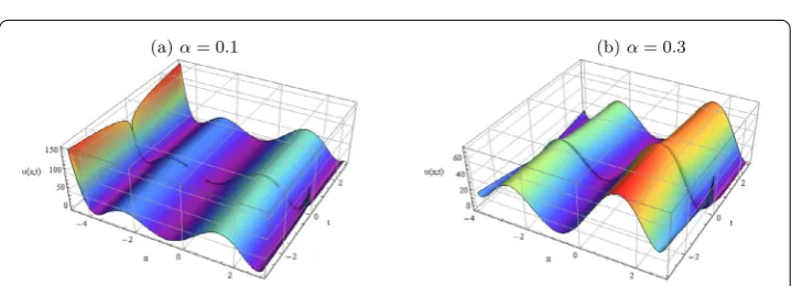
Figure 2The effect ofαon the 3D solitary wave solution of equation (5.10) at different values ofα= 0.1, 0.3 with the suitable parametersk= 0.3,p= 0.2,q= 0.7,r= 0.3,a0= 6,a1= 1.7
whereM=max{3kρ,2aρ, 12dp2},ρ=bp2+c(q2+r2). Now, consider another power series,
S(ξ) =
∞
n=0
snξn, (5.12)
withsi=|ai|,i= 0, 1. Then we can get
sn+2=M n
m=0
|sm||sn–m|
–
n
m=0 n–m
l=0
|sl||sm–l||sn–m|–|sm||sn–m+2|–|sm+1||sn–m+1|–|sm||sn–m+1|
, (5.13)
wheren= 0, 1, 2, . . . thus, it is easily noted that
|an+2| ≤sn+2 this leads to|an| ≤sn,
con-vergence. Then, we write this series in the following form:
S(ξ) =s0+s1ξ+ ∞
n=2
snξn
=s0+s1ξ+M n
m=0
|sm||sn–m|
–
n
m=0 n–m
l=0
|sl||sm–l||sn–m|–|sm||sn–m+2|–|sm+1||sn–m+1|–|sm||sn–m+1|
ξn+2
=s0+s1ξ+M
S2(ξ)ξ2–S3(ξ)ξ2– 2(S–s0)(S–s0)
.
Consider an implicit functional system with respect to the independent variableξ as fol-lows:
ϑ(ξ,S) =S–s0–s1ξ–M
S2(ξ)ξ2–S3(ξ)ξ2– 2(S–s0)(S–s0)
, (5.14)
sinceϑis an analytic in a neighborhood of (o,s0), whereϑ(o,s0) = 0 and,∂ϑ∂S(o,s0)= 0.
Theorem([59]) Let f be a℘-mapping of an open set E⊂sn+minto Sn,such that f(a,b) = 0
for some point(a,b)∈E.Assume that A=f(a,b)and Axis invertible.Then the following
properties hold in the open sets U⊂sn+mand W⊂Smwith(a,b)∈U and b∈W.
(i) For eachy∈W,there exists a uniquexsuch that(x,y)∈Uandf(x,y) = 0. (ii) Ifxis defined to beg(y),then
g(b) =a,
fg(y),y= 0 (y∈W),
g(b) = –(Ax)–1Ay,
where g is a℘-mapping ofWintoSn.
(iii) The function g is implicitly defined by(ii).
One can see that S=S(ξ)is analytical in a neighborhood of the point(o,s0)and has positive
radius.It shows that the power series Eq. (5.5)is convergent in a neighborhood of the point (o,s0).
6 The modified trial equation method for Eq. (1.1)
In this section, we gave a brief description of the modified trial method that was proposed by Liu [60,61]; some authors [62–64] improved this method. Now, let us consider the time FPDEs, say in the four variablesx,y,zandt. In the following we give the main steps of the modified trial method and we obtain some traveling wave solutions of Eq. (1.1):
Step 2: Take the trial equation as follows:
ψ= F(ψ) G(ψ)=
n i=0Aiψi l
j=0Bjψj
=A0+a1ψ+A2ψ
2+· · ·+A nψn
B0+B1ψ+B2ψ2+· · ·+Blψl
,
ψ=F(ψ)(F
(ψ)G(ψ) –F(ψ)G(ψ))
G3(ψ) ,
(6.1)
whereFandGare polynomials inψ. On substituting (6.1) into (5.4) yields an equation of
Ω(ψ) of polynomial inψ
Ω(ψ) =psψs+· · ·+p1ψ+p0,
we found a relation betweennandlaccording to the balance principle and determined some values of them.
Step 3: Setting the coefficients ofΩ(ψ) to zero yields a system of algebraic equations:
pi= 0, i= 0, 1, . . . ,s.
By solving the obtained system of algebraic equations, we can determine the values of A0, . . . ,AnandB0, . . . ,Bl.
Step 4: Rewrite Eq. (5.11) by the following integral form:
ξ–ξ0=
F(ψ)
G(ψ)dψ, (6.2)
whereξ0is the constant of integration. When we classify the roots ofF(ψ) using the
com-plete discrimination system, we obtain the analytical solutions of Eq. (1.1).
Now, applying the modified trial equation method for the (3 + 1)-dimensional time-fractional SZKB equation with the wave transformation defined by Eq. (5.2), by employing (6.1), (6.2), and using the balance principle yieldsn=l+ 2. This resolution procedure was applied and we obtained results as follows.
Case 1: If we takel= 0, thenn= 2, and
ψ=A0+A1ψ+A2ψ
2
B0
,
ψ=(A1+ 2A2ψ)(A0+A1ψ+A2ψ
2)
B2 0
,
(6.3)
thus, we have a system of algebraic equations from the coefficients of polynomial ofu. Solving this system, we get
A0= 0, A2= –
aB0
6dp, r=±
–bp
2+cq2
c , k= –
4dp2A1
B0
.
Substituting from the above coefficients into (6.2) and integrating, we get the solutions to (5.4), as follows:
ξ–ξ0=
B0
A2ψ2+a1ψ
this implies
ψ(ξ) = 3kB0
2p(6dPexp(±4dpk2B
0(ξ–ξ0)) –aB0)
, (6.5)
thus,
u(x,y,z,t) =
3kB0
2p(6dPexp(± k
4dp2B0(px+qy+rz– kt α
Γ(1+α)–ξ0)) –aB0) 2
. (6.6)
For simplicity, takeξ0= 0,A1=A2= 1 then the solution Eq. (6.6) is reduced to the following
solution:
u(x,y,z,t) =
1
exp(γ(px+qy+rz–Γkt(αα+1))) – 1
2
, (6.7)
where γ =±A1
B0. We represent the solution defined by Eq. (6.7) using the 2D plot, see Fig.3b, and the 3D plots, see Fig.3a and Fig.4.
Figure 3(a) The effect ofαon the 3D double-layer solution of equation (6.7) with a fixed timetand the parametersk= 0.3,p= 0.2,q= 0.2. (b) The corresponding 2D plot of (a) with the same parameters
Case 2: If we takel= 1, thenn= 3, and
ψ=A0+A1ψ+A2ψ
2+A 3ψ3
B0+B1ψ
,
ψ=A0+A1ψ+A2ψ2+A3ψ3
B0+B1ψ
A1+ 2A2ψ+ 3A3ψ2
–B1
A0+A1ψ+A2ψ2+A3ψ3
/(B0+B1ψ)3,
(6.8)
thus, we have a system of algebraic equations from the coefficients of polynomial ofu. Solving this system, we get
A0= 0, A2=
6dpA1B1–aB20
6dpB0
, A3= –
aB1
6dp,
k=4dp
2A 1
B0
, r=±
–bp
2+cq2
c .
Substituting from the above coefficients into Eq. (6.8) and integrating, we get the solutions to Eq. (5.4), as follows:
ξ–ξ0=
B0+B1u
A3ψ3+A2ψ2+a1ψ
dψ, (6.9)
this implies
ξ–ξ0= –
1 2A1
B0ln
A1+ψ(A2+A3ψ)
– 2B0ln(ψ)
+ 1
σ
2(A2B0– 2A1B1)tan–1
A2+ 2A3ψ
σ
, (6.10)
whereσ=4A1A3– 2A22. Substituting the values ofAi,i= 1, 2, 3, thus
ψ(ξ) =
3k 2ap+exp(k(ξ0–ξ)
4dp2 )
, (6.11)
whereξ=px+qy+rz–Γ(ktαα+1).
For simplicity, takeξ0= 0 then the solution Eq. (6.11) is reduced to the following
solu-tion:
u(x,y,z,t) =
3k
2ap+exp(–k(px+qy+rz– ktα Γ(α+1))
4dp2 )
2
. (6.12)
We represent the solution defined by Eq. (6.12) using the 2D plot, see Fig.5b, and the 3D plots, see Fig.5a and Fig.6.
7 Conclusion
Figure 5(a) The effect ofαon the 3D double-layer solution of equation (6.12) with a fixed timetand the parametersk= 0.3,p= 0.2,q= 0.2. (b) The corresponding 2D plot of (a) which shows that when the value of αincreases the interval of the stability of the solution also increases
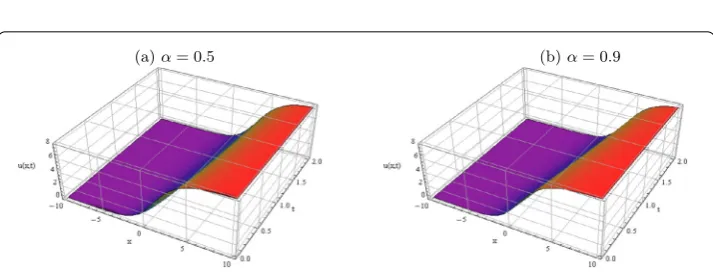
Figure 6The 3D double-layer solution of equation (6.12) at different values ofα= 0.5, 0.9 with the suitable parametersk= 0.3,p= 0.2,q= 0.2
waves (DIAWs) in a magnetized dusty plasma. The Lie point symmetries were applied successfully to the study of the (3 + 1)-dimensional time-fraction Schamel–Zakharov– Kuznetsov–Burgers equation. Based on the Riemann–Liouville derivatives, we deduced the corresponding vector fields, which helped us to construct the symmetry reductions of the time-fractional SZKB equation. Furthermore, we obtained four kinds of conserva-tion laws with independent variables laying the foundaconserva-tion of Lie point symmetries. Also, we constructed a new set of analytical solutions via two powerful methods, which are the explicit power series method and the modified trial equation method. Moreover, to intro-duce a better understanding of the dynamics of these solutions, we provided their graphic analysis of Eq. (1.1). As shown in Fig.3, It was noticed that the solutionu(x,y,z,t) defined by Eq. (6.7) remained stable for –4.35 <x< 2.75 and has a singularity outside this interval. It can easily be observed in Figs.4and6that the solutions are in line with the values of
α, it means that the singularity becomes clearer when the value ofαdecreases. Thus, we expect that the obtained results might serve as the explanation of the physical meaning of the time-fractional SZKB equation with more accuracy. However, we can extend the symmetry analysis to the time-space fractional (3 + 1)-dimensional Schamel–Zakharov– Kuznetsov–Burgers equation where that work may be presented later elsewhere.
Acknowledgements
Funding
This research work is not supported by any funding agencies.
Competing interests
The authors declare that no competing interests exist.
Authors’ contributions
The authors declare that the work was realized in collaboration with the same responsibility. All authors read and approved the final paper.
Publisher’s Note
Springer Nature remains neutral with regard to jurisdictional claims in published maps and institutional affiliations.
Received: 12 July 2019 Accepted: 9 October 2019
References
1. Biswas, A., Mirzazadeh, M., Eslami, M.: Dispersive dark optical soliton with Schödinger–Hirota equation (G/G)-expansion approach in power law medium. Optik125(16), 4215–4218 (2014)
2. Eslami, M., Ebrahimi, M.: Explicit solutions of nonlinear (2 + 1)-dimensional dispersive long wave equation. J. King Saud Univ., Sci.24(1), 69–71 (2012)
3. Liu, J., Eslami, M., Rezazadeh, H., Mirzazadeh, M.: Rational solutions and lump solutions to a non-isospectral and generalized variable-coefficient Kadomtsev–Petviashvili equation. Nonlinear Dyn.95(2), 1027–1033 (2019) 4. Mirzazadeh, M., Eslami, M., Biswas, A.: Dispersive optical solitons by Kudryashov’s method. Optik, Int. J. Light Electron
Opt.125(23), 6874–6880 (2014)
5. Mirzazadeh, M., Eslami, M., Zerrad, E., Mahmood, M., Biswas, A., Belic, M.: Optical solitons in nonlinear directional couplers by sine–cosine function method and Bernoulli’s equation approach. Nonlinear Dyn.81(4), 1933–1949 (2015)
6. Nazarzadeh, A., Eslami, M., Mirzazadeh, M.: Exact solutions of some nonlinear partial differential equations using functional variable method. Pramana81(2), 225–236 (2013)
7. Mirzazadeh, M., Eslami, M.: Exact solutions of the Kudryashov–Sinelshchikov equation and nonlinear telegraph equation via the first integral method. Nonlinear Anal., Model. Control17(4), 481–488 (2012)
8. Eslami, M., Neirameh, A.: New exact solutions for higher order nonlinear Schrödinger equation in optical fibers. Opt. Quantum Electron.50(1), Article ID 47 (2018)
9. Biswas, A., Mirzazadeh Eslami, M.: Optical solitons with Biswas–Milovic equation for power law and dual-power law nonlinearities. Nonlinear Dyn.83(1–2), 731–738 (2016)
10. Mirzazadeh, M., Eslami, M., Biswas, A.: Trial solution technique to chiral nonlinear Schrodinger’s equation in (1 + 2)-dimensions. Nonlinear Dyn.85(2), 813–816 (2016)
11. Song, F., Yu, Z., Yang, H.: Modeling and analysis of fractional neutral disturbance waves in arterial vessels. Math. Model. Nat. Phenom.14, Article ID 301 (2019)
12. Yang, H., Guo, M., He, H.: Conservation laws of space-time fractional mZK equation for Rossby solitary waves with complete Coriolis force. Int. J. Nonlinear Sci. Numer. Simul.20, 17–32 (2019)
13. Oldham, K.B., Spanier, J.: The Fractional Calculus, pp. 1–84. Academic Press, New York (1974)
14. Samko, S., Kilbas, A.A., Marichev, O.: Fractional Integrals and Derivatives: Theory and Applications. Gordon & Breach, Yverdon (1993)
15. Miller, K.S., Ross, B.: An Introduction to the Fractional Calculus and Fractional Deferential Equations. Wiley, New York (1993)
16. Kiryakova, V.: Generalised Fractional Calculus and Applications. Pitman Research Notes in Mathematics, vol. 301. Longman, London (1994)
17. Ahmad, B., Ntouyas, S.K., Alsaedi, A.: On a coupled system of fractional differential equations with coupled nonlocal and integral boundary conditions. Chaos Solitons Fractals83, 234–241 (2016)
18. Biala, T.A., Jator, S.N.: Block implicit Adams methods for fractional differential equations. Chaos Solitons Fractals81, 365–377 (2015)
19. Shah, K., Khalil, H., Khan, R.A.: Investigation of positive solution to a coupled system of impulsive boundary value problems for nonlinear fractional order differential equations. Chaos Solitons Fractals77, 240–246 (2015) 20. Ren, Y., Tao, M., Dong, H., Yang, H.: Analytical research of (3 + 1)-dimensional Rossby waves with dissipation effect in
cylindrical coordinate based on Lie symmetry approach. Adv. Differ. Equ.2019, Article ID 13 (2019) 21. Abdelkawy, M.A., Zaky, M.A., Bhrawy, A.H., Baleanu, D.: Numerical simulation of time variable fractional order
mobile–immobile advection–dispersion model. Rom. Rep. Phys.67, 773–791 (2015)
22. Wang, Q.: Homotopy perturbation method for fractional KdV Burgers equation. Chaos Solitons Fractals35, 843–850 (2008)
23. Gupta, P.K., Singh, M.: Homotopy perturbation method for fractional Fornberg–Whitham equation. Comput. Math. Appl.61, 250–254 (2011)
24. Ray, S.S.: Analytical solution for the space fractional diffusion equation by two-step Adomian decomposition method. Commun. Nonlinear Sci. Numer. Simul.14, 1295–1306 (2009)
25. Nazari, D., Shahmorad, S.: Application of the fractional differential transform method to fractional-order integro differential equations with nonlocal boundary conditions. J. Comput. Appl. Math.234, 883–891 (2010) 26. Gupta, P.K.: Approximate analytical solutions of fractional Benney–Lin equation by reduced differential transformmethod and the homotopy perturbation method. Comput. Math. Appl.61, 2829–2842 (2011) 27. Abdel-Salam, E.A., Yousif, E.A.: Solution of nonlinear space-time fractional differential equations using the fractional
28. Zhang, S.H., Zhang, Q.: Fractional sub-equation method and its applications to nonlinear fractional PDEs. Phys. Lett. A
375, 1069–1073 (2011)
29. Abdelkawy, M.A., El-Kalaawy, O.H., Al-Denari, R.B., Biswas, A.: Application of fractional subequation method to nonlinear evolution equations. Nonlinear Anal., Model. Control23, 710–723 (2018)
30. Gepreel, K.A., Mohamed, M.S.: Analytical approximate solution for nonlinear space-time fractional Klein–Gordon equation. Chin. Phys. B22, 201–211 (2013)
31. Yulita Molliq, R., Batiha, B.: Approximate analytic solutions of fractional Zakharov–Kuznetsov equation by fractional complex transform. Int. J. Eng. Technol.1, 1–13 (2012)
32. Asiru, M.A.: Sumudu transform and the solution of integral equations of convolution type. Int. J. Math. Educ. Sci. Technol.32, 906–910 (2001)
33. Rana, M.A., Siddiqui, A.M., Ghori, Q.K., Qamar, R.: Application of He’s homotopy perturbation method to Sumudu transform. Int. J. Nonlinear Sci. Numer. Simul.8, 185–190 (2007)
34. Eltayeb, H., Kylycman, A.: On some applications of a new integral transform. Int. J. Math. Anal.4, 123–132 (2010) 35. Gazizov, R.K., Kasatkin, A.A., Lukashchuk, S.Y.: Symmetry properties of fractional diffusion equations. Phys. Scr.36, 1–5
(2009)
36. Bluman, G.W., Kumei, S.: Symmetries and Differential Equations, pp. 31–89. Springer, New York (1989) 37. Olver, P.J.: Application of Lie Groups to Differential Equations, pp. 2–24. Springer, New York (1993) 38. Ibragimov, N.H.: Elementary Lie Group Analysis and Ordinary Differential Equations. Wiley, Chichester (1999) 39. Lukashchuk, S.Y.: Conservation laws for time-fractional subdiffusion and diffusion-wave equations. Nonlinear Dyn.23,
153–163 (2015)
40. Abdullahi, R.A., Muatjetjeja, B.: Conservation laws and exact solutions for a 2D Zakharov–Kuznetsov equation. Appl. Math. Lett.1, 109–117 (2015)
41. El-Kalaawy, O.H.: Variational principle, conservation laws and exact solutions for dust ion acoustic shock waves modeling modified Burger equation. Comput. Math. Appl.72, 1031–1041 (2016)
42. El-Kalaawy, O.H.: Modulational instability: conservation laws and bright soliton solution of ion-acoustic waves in electron-positron-ion-dust plasmas. Eur. Phys. J. Plus133, Article ID 58 (2018)
43. El-Kalaawy, O.H.: New: variational principle-exact solutions and conservation laws for modified ion-acoustic shock waves and double layers with electron degenerate in plasma. Phys. Plasmas24, 308 (2017)
44. El-Kalaawy, O.H., Moawad, S.M., Wael, S.: Stability: conservation laws, Painlevé analysis and exact solutions for S-KP equation in coupled dusty plasma. Results Phys.7, 934–946 (2017)
45. Adem, A.R., Khalique, C.M.: Symmetry reductions exact solutions and conservation laws of a new coupled KdV system. Commun. Nonlinear Sci. Numer. Simul.17, 3465–3475 (2012)
46. Noether, E.: Invariant variation problems. Transp. Theory Stat. Phys.1, 186–207 (1971) 47. Ibragimov, N.H.: A new conservation theorem. J. Math. Anal. Appl.28, 311–333 (2007)
48. Lu, C., Xie, L., Yang, H.: Analysis of Lie symmetries with conservation laws and solutions for the generalized (3 + 1)-dimensional time fractional Camassa–Holm–Kadomtsev–Petviashvili equation. Comput. Math. Appl.77, 3154–3171 (2019)
49. Yang, H., Sun, J., Fu, C.: Time-fractional Benjamin–Ono equation for algebraic gravity solitary waves in baroclinic atmosphere and exact multi-soliton solution as well as interaction. Commun. Nonlinear Sci. Numer. Simul.71, 187–201 (2019)
50. El-Kalaawy, O.H., Engy, A.A.: Shock waves, variational principle and conservation laws of a
Schamel–Zakharov–Kuznetsov–Burgers equation in a magnetised dust plasma. Z. Naturforsch. A73, 693–704 (2018) 51. Hadjaz, I., Tribeche, M.: Alternative dust-ion acoustic waves in a magnetized charge varying dusty plasma with
nonthermal electrons having a vortex-like velocity distribution. Astrophys. Space Sci.351, 591–598 (2014) 52. Sahoo, S., Saha Ray, S.: Analysis of Lie symmetries with conservation laws for the (3 + 1) dimensional time-fractional
mKdV-ZK equation in ion-acoustic waves. Nonlinear Dyn.90, 1105–1113 (2017)
53. Gazizov, R.K., Kasatkin, A.A., Lukashcuk, S.Y.: Continuous transformation groups of fractional differential equations. Vestn., UGATU9, 125–135 (2007)
54. Sahadevan, R., Bakkyaraj, T.: Invariant analysis of time fractional generalized Burgers and Korteweg–de Vries equations. J. Math. Anal. Appl.393, 341–347 (2012)
55. Baleanu, D., Diethelm, K., Scalas, E., Trujillo, J.J.: Fractional Calculus: Models and Numerical Methods. World Scientific, Singapore (2012)
56. Uchaikin, V., Sibatov, R.: Fractional kinetics in solids: anomalous charge transport in semiconductors. In: Dielectrics and Nanosystems, vol. 9, pp. 401–402. World Scientific, Singapore (2013)
57. Galaktionov, V.A., Svirshchevskii, S.R.: Exact Solutions and Invariant Subspaces of Nonlinear Partial Differential Equations in Mechanics and Physics. Chapman & Hall/CRC, Boca Raton (2006)
58. Tian, S.F., Zhang, H.Q.: On the integrability of a generalized variable-coefficient Kadomtsev–Petviashvili equation. J. Phys. A132, 212–246 (2012)
59. Rudin, W.: Principles of Mathematical Analysis, pp. 223–228. China Machine Press, Beijing (2004)
60. Liu, C.S.: Trial equation method to nonlinear evolution equations with rank inhomogeneous: mathematical discussions and its applications. Commun. Theor. Phys.45, 219–223 (2006)
61. Liu, C.S.: New exact envelope traveling wave solutions of high-order dispersive cubic-quintic nonlinear Schrödinger equation. Commun. Theor. Phys.44, 799–801 (2005)
62. Jun, C.Y.: Cubic structures applied to ideals of BCI-algebras. Comput. Math. Appl.62, 3987–3996 (2011) 63. Pandir, Y., Gurefe, Y., Kadak, U., Misirli, E.: Classification of exact solutions for some nonlinear partial differential
equations with generalized evolution. Abstr. Appl. Anal.2012, Article ID 478531 (2012)