A preci
s
e hypocenter determination method u
s
ing network correlation
coefficient
s
and it
s
application to deep low-frequency earthquake
s
Kazuaki Ohta and Satoshi Ide
Department of Earth and Planetary Science, University of Tokyo, 7-3-1 Hongo, Bunkyo, Tokyo 113-0033, Japan
(Received March 13, 2008; Revised April 24, 2008; Accepted April 30, 2008; Online published September 8, 2008)
A knowledge of the precise locations of deep low-frequency earthquakes (LFEs) along subduction zones is essential to be able to constrain the spatial extent of various slow earthquakes and the underlying physical processes. We have developed a hypocenter determinationmethod that utilizes the summed cross-correlation coefficient overmany stations, denoted a network correlation coefficient (NCC). The method consists of two parts: (1) an estimation of relative hypocenter locations for every pair of events by a grid search, and (2) a linear least squares inversion for self-consistent relative hypocenter locations for the initial centroid. We have applied thismethod to ten LFEs in the Tokai region, Japan. Statistically significant values ofNCC indicate the relative locations formany pairs, which in turn determine the self-consistent locations. While the catalog depths are widely distributed, the relocated hypocenters fall within a 2-kmdepth range, which implies that LFEs in the Tokai region occur on the plate interface, similar to LFEs in western Shikoku.
Key words:Low-frequency earthquakes, precise hypocenter determination, cross-correlation coefficient, Nankai subduction zone, Tokai region.
1.
Introduction
Since the discovery of low-frequency tremors along the Nankai subduction zone in western Japan by Obara (2002),
many studies focused on studying various unusual earth-quakes in this area, such as low-frequency earthearth-quakes (LFE) (Katsumata and Kamaya, 2003; Shellyet al., 2006), very low-frequency earthquakes (Itoet al., 2007), and slow slip events (Hirose and Obara, 2005). These unusual events
may provide a clue to understanding subduction in general because similar phenomena are widely observed (Schwartz and Rokosky, 2007; Ideet al., 2007a).
Of the group classified as slow earthquakes, LFEs have been studied with relatively precise event locations due to their frequent occurrence and isolated signals. Shellyet al.
(2006) determined the locations of LFE in western Shikoku using double-difference tomography and relative hypocen-ter location (Zhang and Thurber, 2003) and found that the hypocenters are distributed at a depth of 30–35 km, parallel to intraslab earthquakes, suggesting that these events occur on the plate boundary. Shellyet al.(2007a, b) also dem on-strated that deep low-frequency tremors can be represented as a swarm of LFEs. Consequently, a knowledge of the properties of LFEs would lead to a better understanding of the whole tremor sequence.
Unfortunately, precise locations are not available in other regions of the Nankai trough, such as the eastern Shikoku, Kii peninsula, and Tokai regions, where LFE hypocenters determined by Japan Meteorological Agency (JMA) have a wide depth distribution. In the Tokai region, the depth
dis-Copyright cThe Society of Geomagnetismand Earth, Planetary and Space Sci-ences (SGEPSS); The Seismological Society of Japan; The Volcanological Society of Japan; The Geodetic Society of Japan; The Japanese Society for Planetary Sci-ences; TERRAPUB.
tribution ranges from20 to 50 km(Fig. 1) and resembles the tremor source distribution determined by Kaoet al.(2005) in the Cascadia subduction zone. Since the wide depth dis-tribution suggests a different physical interpretation, such as fluidmovement in the overriding plate, the important ques-tion is whether or not the apparent wide depth distribuques-tion of LFEs along the Nankai subduction zone is real.
For signals in noisy records, the summation of cross-correlation coefficients for network stations, denoted the network correlation coefficient (NCC), is a useful tool, as demonstrated by Shellyet al.(2007a, b). These researchers detectedmany small LFEs in a continuous tremor sequence using NCC and known LFEs as template events. Their
method, calledmatched filter analysis (Gibbons and Ring-dal, 2006), can bemodified to determine the relative loca-tion between event pairs. In this paper, we report our devel-opment of a new hypocenter determinationmethod based on this concept. This newmethod is applied to a small set of real data, LFEs in the Tokai region (Fig. 1), to verify its effectiveness.
2.
Method
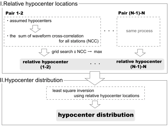
2.1 Overview
The newmethod consists of twomain steps, as illustrated in Fig. 2. First, we estimate the relative hypocenter location for each pair of events by maximizing the summation of waveformcross-correlation, or NCC, for all stations. We then determine a set of hypocenter locations that are con-sistent with the relative locations by solving a least square problem.
2.2 Determination of relative hypocenter location be-tween a pair of events
We first determine the relative hypocenter location be-tween a pair of earthquakes, eventsi and j. The eventi
34.8
Fig. 1. (Top) Map showing the study area and the locations of LFEs (red crosses) and regular intraplate earthquakes (blue circles), determined by JMA. LFEs used for example are shown within the small gray square. The location of study area in Japan is shown in the inset. Triangles are stations. (Bottom) Cross-sectional view of the hypocenter distribution within the thick green rectangular oriented in the plate subduction di-rection.
is used as a reference event, with known location and ori-gin time that are tentatively assumed to be the JMA catalog values. Ground velocity waveformin thel-th direction from
the eventi recorded at a seismic stationn,uiln(t), is digi-the digi-theoretical travel time of a body wave fromthe source locationxi0to the stationxn,t(x0i,xn), and a presignal time
Tpre. The other event, j, is a target event. Its seismogram is similarly prepared with a time shift calculated fromthe relative hypocenter location between two events,xi j, and
This is the network correlation coefficient, NCC, defined by Gibbons and Ringdal (2006) and used by Shellyet al.
(2007a, b) to detect LFEs in a tremor sequence.
TheNCCis high only when waveforms fromtwo events correlate for all stations and components. Therefore, the relative location, xNCC
i j , is determined by the maximum
of the NCC. Since theNCC hasmany localmaxima that can be a source of uncertainty, we determine the global
maximumusing a grid search. Applying this procedure to every pair ofNevents yieldsN×(N−1)relative locations, x12NCC, . . . , xi jNCC, . . . , x
NCC N N−1.
2.3 Least-squares inversion for self-consistent hypocenter locations
Once relative locations between events aremeasured pre-cisely and the location of one event is given, the absolute locations of all events are in principle automatically
deter-mined. However, the uncertainty of the relative hypocenter locations is neither negligible nor homogeneous. We as-sume that the relative locations for all combinations forma data vector with Gaussian errors, each of which has a vari-ance depending on the value of the NCC. Unknown pa-rameters are hypocenter locationsxm(m = 1, . . . ,N),
de-wherewi jis a weighting factor. Since the absolute location
is not constrained by the above equation, we also assume that the centroid of the hypocenters is unchanged fromthe catalog value so that
The weighting factor is calculated based on the proba-bility that a relative location is correct. Although a large
maximumof NCC generallymeans high reliability, even waveforms of Gaussian noisemay occasionally show a very large value in numerous iterations. If theNCCismeasured fromdiscrete time series of M samples of Gaussian white noise with a unit standard deviation atNstations, theNCC
Fig. 2. A schematic diagramshowing themain two steps of the newmethod in the case of determining hypocenter distribution ofNevents.
if calculations at different grid points are independent. For example, in a grid search for 1004 points, 100 grid points in three-dimensional (3D) space and time, the maximum
exceeds 5σNCCand 6σNCC, with probabilities of about 100%
and 10%, respectively. The standard deviation ofNCC for real data ismeasured fromNCCvalues at all grid points.
When the ratio between themaximumand the standard deviation of the NCC isri j for the event pairi and j, we
assume the variance of the estimation error to be the sumof variances of noise and signals,
σ2
d(ri j)=PNg(ri j)σN2+(1−PNg(ri j))σS2, (7)
whereσ2
S andσN2 are the variances of signals and random noises, respectively. It should be noted that even in the case of identical signals, because we adopted a grid search scheme, there is a quantization error that is dependent on the grid point intervall. On the other hand, the variance of noise depends on the size of search space, L, in which any points are equally selected as the target location. Thus, σ2
NandσS2are respectively written as
σ2
The reciprocal of this variance, σ2
d(ri j), is the weighting factorwi jin Eq. (4).
3.
Application to LFE
s
in the Tokai Region
3.1 Study area and waveform data
We apply this method to LFEs in the Tokai region (Fig. 1). More than 1000 LFEs have been detected and lo-cated by JMA between 2002 and 2007, and the locations listed in the catalog are widely distributed. Before apply-ing the newmethod, we attempted to determine hypocenter locations using the double-differencemethod (Waldhauser and Ellsworth, 2000) with cross correlation, similar to the analysis of LFEs carried out in western Shikoku by Shelly
et al. (2006). However, few cross-correlation coefficients exceed 0.7, a threshold value used in Shellyet al.(2006), and we were unable to obtain reliable results.
As a first small data set, we selected ten events fromthe original data set of 1000 LFEs. These events have rela-tively large amplitude and impulsive waveforms and oc-curred within a small area (Fig. 1). The data are three-component velocity seismograms observed at the Hi-net stations. We then calculated the cross correlation using the vertical component of theP-wave and two horizontal com -ponents of the S-wave. Each seismogramis bandpass fil-tered between 2 and 8 Hz. The number of stations available for each event pair is different and averages about ten. The time window used for calculating a cross correlation is from
1.5 s before to 2.5 s after the theoretical P- orS-wave ar-rival times, which are calculated assuming a horizontally layered structure based on local seismic reflection and re-fraction surveys (Iidakaet al., 2003).
3.2 Relative hypocenter location determined byNCC
We first determined the relative hypocenter locations for all combinations of these ten events. We assume that the differences of latitude, longitude, and depth between two events are within 0.1◦, 0.1◦, and 10 km, respectively, and search the locationxNCC
i j , which gives themaximumNCC
in this range. The range of the origin time shift ti j is
between −2 and +2 s. A grid search for xi j and ti j
revealed themaximum, with grid point intervals of 0.001◦, 0.001◦, 0.1 km, and 0.04 s, in latitude, longitude, depth, and time directions, respectively.
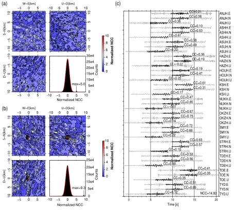
Figure 3 shows the spatial distributions and histograms ofNCC for two pairs of events. In the first case (Fig. 3(a)), themaximumis fivefold the standard deviation,σNCC, and
the localmaxima of similar values are widely distributed in the search space. As already explained, themaximum
of such low values is well explained by Gaussian noise and
many iterative calculations. Therefore, this estimation is almostmeaningless. On the other hand, in the second ex-ample (Fig. 3(b)), the localizedmaximumis 9.3σNCC. The
05
Fig. 3. The contourmap and histogramofNCCfor the event pair which have (a) a statistically insignificantmaximumvalue ofNCC(fivefold the standard deviation) and (b) a statistically highmaximum(9.3-fold). In the contourmaps, themaximumNCCfor temporal grids at each spatial grid point is shown, normalized by the standard deviation. The red line of each histogrampanel shows a Gaussian distribution. (c) For the highNCC
maximumpair shown in (b), waveforms of the reference event (black) and the target event (gray) are compared for each component of 12 Hi-net stations. The correlation coefficient (CC) is shown for each trace, and the total sum,NCC, is shown in the lower right of the panel. Station names and components are written to the right of each trace.
(Fig. 3(c)), which even in the best case prevents the appli-cation of standardmethods, such as the double-difference technique. Nevertheless, themaximumNCCis statistically significant; the probability that Gaussian noise leads to this value,∼5.8×10⁻¹⁰, is obtained using Eq. (6). Therefore, this location of the maximum NCC [(latitude, longitude, depth)=(−0.011◦,−0.009◦,−0.1 km)] certainly indicates the relative location between two events. These values are slightly different fromthe relative location in the catalog, (−0.0030◦, 0.0077◦,−0.67 km). When we switch the ref-erence and the target, the maximum NCC of 8.9σNCC is
obtained at (0.011◦, 0.009◦, 0 km), which is almost the op-posite.
Among 90 pairs of events, 21 and 35 combinations have
NCC larger than 7σNCC and 6.5σNCC, with probabilities
given by Eq. (6) of about 0.1% and 3%, respectively. 3.3 Relocation
A linear inversion of the relative locations with variances given by Eq. (7) determines the self-consistent hypocenter
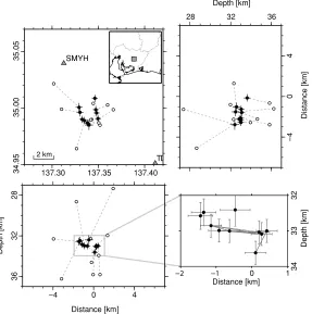
locations of the ten LFEs, as shown in Fig. 4. The hypocen-ter distribution ismore concentrated than the catalog loca-tions of JMA, particularly in terms of depth, which spans a 2-kmrange, suggesting that the depth variation in the cata-log is due to errors in the picks and velocitymodel.
Figure 4 also shows that the LFEs are separated into two groups: amain group of seven events and a two-event group to the west of the main group. Within each group, the LFEs are strongly connected to each other, as shown by “bonds”—i.e., highNCC values larger than 7σNCC, in the
lower-right panel of Fig. 4. In themain group, several bonds ofmore than a 1-kmdistance separate events into two sub-groups, with an east-west distribution. The location of one event that has no highNCC bond with other events is not well determined. The shallow depth of this event, 27.4 km, in the JMA catalog suggests that the true locationmay be far fromthose of the other events. Another possibility is that themechanismof this event is different. We assume that the
34.95
35.00
35.05
137.30 137.35 137.40 SMYH
TD 2 km
36
32
28
Depth [km
]
0 4
Distance [km]
04
Distance [km
]
28 32 36
Depth [km]
34
33
32
Depth [km]
0 1
Distance [km]
Fig. 4. The hypocenter locations of ten LFEs used for the analysis. A black and white circle connected by a dashed line are the relocated and the catalog locations for one event. Crosses show the standard deviation of themodel parameters. The close-up panel shows the connection between pairs that have highly correlated waveforms. A “bond” connects two events that haveNCClarger than 7σNCC.
in Shikoku (Ide et al., 2007b), and while themany statis-tically significantNCC values support this assumption, we cannot exclude the possibility ofmechanismvariation for some events.
4.
Di
s
cu
ss
ion and Conclu
s
ion
When we calculated the cross correlation of seismic waves between two events simultaneously for many sta-tions, we were able to precisely evaluate the relative loca-tion even in the presence of noise. Although the value of the correlation coefficient is small at each station, the sum, the network correlation coefficient (NCC), acquires a sta-tistically significant value, which cannot be explained by Gaussian noise. The newmethod is robust and applicable for the events with a low signal-to-noise ratio if the source
mechanisms are similar.
In this paper, we apply thismethod to ten LFEs in the Tokai region. The relocated hypocenters are more con-centrated than those in the JMA catalog, suggesting that the apparent wide distribution in the catalog is an artifact. Since the subducting Philippine Sea plate changes strike be-neath the study area, suggesting some complexity, and the assumed structure is just 1D, it is difficult to be sure pre-cisely where these events occur; however, the localization in depth suggests that these LFEs occur along some irregular-ity; the plate interface is an obvious candidate. Despite ap-parent differences in the original catalog and the existence of short- and very long-termslow slip events (Hirose and Obara, 2006; Miyazakiet al., 2006), LFEs in the Tokai re-gionmay have the same characteristics as those in western Shikoku, where LFEs are considered to be shear slip on the
plate interface (Shellyet al., 2006; Ideet al., 2007b). Appli-cation to large event sets will increase the number of bonds andmay connect the separate groups in this study. Since the
method is applicable to all events with a low signal-to-noise ratio, we expect to be able to apply thismethod not only to LFEs but also to low-frequency tremors.
Acknowledgments. We are grateful to Greg Beroza for his en-lightening comments. We thank David Schaff and Yoshihiro Ito for their careful and constructive reviews. This work is supported by Grant-in-Aid for Scientific Research, Ministry of Education, Sports, Science and Technology, Japan and JSPS Bilateral Joint Project.
References
Gibbons, S. J. and F. Ringdal, The detection of lowmagnitude seismic events using array-based waveformcorrelation,Geophys. J. Int.,165, 149–166, 2006.
Hirose, H. and K. Obara, Repeating short- and long-termslow slip events with deep tremor activity around the Bungo channel region, southwest Japan,Earth Planets Space,57, 961–972, 2005.
Hirose, H. and K. Obara, Short-term slow slip and correlated tremor episodes in the Tokai region, central Japan,Geophys. Res. Lett.,33, L17311, doi:10.1029/2006GL026579, 2006.
Ide, S., G. C. Beroza, D. R. Shelly, and T. Uchide, A scaling law for slow earthquakes,Nature,447, 76–79, 2007a.
Ide, S., D. R. Shelly, and G. C. Beroza, The mechanismof deep low frequency earthquakes: Further evidence that deep non-volcanic tremor is generated by shear slip on the plate interface,Geophys. Res. Lett.,34, L03308, doi:10.1029/2006GL028890, 2007b.
circum-Pacific subduction zones,Rev. Geophys.,45, RG3004, doi:10. 1029/2006RG000208, 2007.
Shelly, D. R., G. C. Beroza, S. Ide, and S. Nakamula, Low-frequency