R E S E A R C H
Open Access
Impact of spatial sampling frequency offset
and motion blur on optical wireless
systems using spatial OFDM
M. Rubaiyat H. Mondal
Abstract
Pixelated communication systems can convey high-speed data over optical wireless channels by using
spatial orthogonal frequency division multiplexing(spatial OFDM) modulation. Two forms of spatial OFDM, spatial asymmetrically clipped optical OFDM (SACO-OFDM) and spatial dc-biased optical OFDM (SDCO-OFDM), have been considered in the literature of pixelated communication. This paper mathematically describes the SACO-OFDM signal and then proposes a power-efficient derivative of SACO-OFDM termed as noise-cancelled spatial OFDM (NCS-OFDM). However, NCS-OFDM and other spatial OFDM systems can be impaired by spatial sampling frequency offset (SSFO) defined as the difference in the number of transmitted and received pixels and by coexisting defocus and motion blur forming an asymmetric point spread function (APSF). In this paper, for the first time, the effects of SSFO and APSF on a spatial OFDM based pixelated system are investigated. Simulation results show that both SSFO and APSF cause phase distortions and attenuation of the data-carrying spatial-subcarriers resulting in bit error rate (BER) degradation. Simulation results also indicate that in the presence of several channel impairments including SSFO and APSF, NCS-OFDM outperforms SACO-OFDM and SDCO-OFDM in terms of power efficiency.
Keywords:Motion blur, Noise, OFDM, Optical wireless communication, Pixels, Pixelated systems, Spatial OFDM
1 Introduction
In recent years, wireless data traffic has experienced enor-mous growth due to the increase in bandwidth-intensive applications such as video streaming, voice over IP and network-attached storage. Consequently, the radio fre-quency (RF) spectrum is becoming more and more con-gested. Multiple-input multiple-output (MIMO) optical wireless communication (OWC) [1–10] is considered as a supplemental technology to RF links for many high data rate applications. MIMO OWC can have either a non-imaging or an non-imaging receiver. Research has shown that MIMO systems using non-imaging concentrators do not perform well at many receiver positions, and conse-quently, little diversity gain is obtained. The use of an im-aging receiver may overcome this problem [8]. One form
of imaging system is pixelated OWC [11–19], where the
term pixelated means that the optical modulator, the
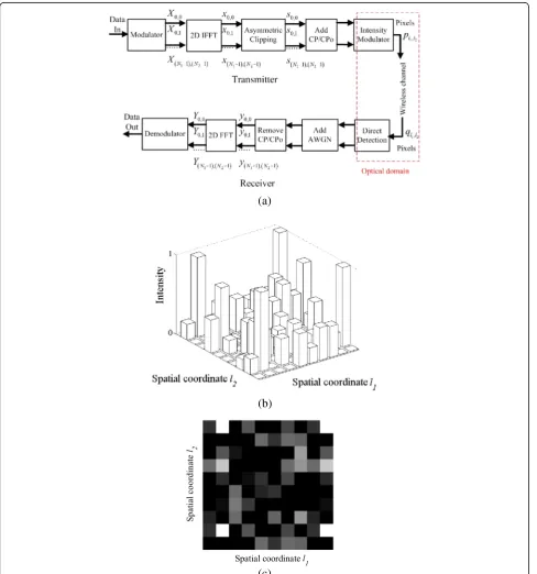
transmitted images and the detector are each composed of a large number of smaller units. Figure 1 illustrates pixelated communication where a number of image frames are used to carry the data. Such a system operates based on image transfer. For pixelated OWC, a pixelated grid of light-emitting diodes (LEDs) or a liquid crystal dis-play (LCD) screen can be used as a transmitter. In addition, arrays of pixel sources found in devices such as TVs, display walls, lighting and electronic billboards may also be considered as such transmitters. On the other hand, an imaging lens along with an array of photodiodes or a stand-alone camera can be used as a receiver [11, 14]. In between the transmitter and the receiver, a two dimen-sional (2-D) optical wireless channel is described by its spatial impulse response known as the point spread func-tion (PSF).
Pixelated systems may provide high transmission rates by exploiting spatial diversity at a large scale. A number of recent proof-of-concept experiments re-ported in [11, 14, 15] have demonstrated the feasibility Correspondence:[email protected]
Institute of Information and Communication Technology (IICT), Bangladesh University of Engineering and Technology (BUET), Dhaka, Bangladesh
of pixelated communication. Such a system has the poten-tial to provide a well-directed secure link for inter-device communication of gigabytes of data. Therefore, these links can be used for a number of near-field communication ap-plications such as mobile advertisements, secure data communication, data transfer in dense high-contention scenarios and vehicle-to-traffic light communication [14]. However, the pixelated transmitter has to be within the field of view of the imaging receiver [11], limiting the ex-tent of user mobility, and thus, systems of this type may not be suitable for some application areas.
In order to transmit data in parallel, a pixelated system
may apply spatial orthogonal frequency division
multi-plexing (spatial OFDM) [11, 14, 18, 20–22], which is essentially an extension of the conventional OFDM
con-cept [23–25] to the 2-D spatial domain. For spatial
OFDM modulation, information is encoded using several orthogonal 2-D subcarriers in the spatial-frequency domain which is the frequency representation of the 2-D image space. Each of the 2-D spatial OFDM frames is transformed into a pixelated image. These images are transmitted into the 2-D optical channel. For pixelated OWC, spatial OFDM exhibits a number of advantages compared to systems that encode data directly in the spatial domain. For instance, the use of spatial OFDM algorithms at the transmitter side allows generating data-carrying images in a way that makes them much robust to 2-D spatial distortions. Consequently, the re-ceiver can apply simple correction algorithms to decode the images [14, 18, 26, 27].
However, the technology of spatial OFDM based pixelated systems is still in its infancy and has to over-come several challenges including power constraints, spatial distortions [18, 27–29] and temporal distortions [16, 30]. Limiting factors such as ambient light [14], spatial perspective distortions [14], spatial rotational error [19] and temporal synchronization problems [16] have been studied in the literature. In recent years, the author of this paper has analysed the effects of spatial
distortions such as defocus blur [28, 29], vignetting [18] and fractional misalignment error [27]. The results re-ported in the above-mentioned previous studies are based on the assumption that the numbers of pixels in the transmitted images and the corresponding received images are the same. In other words, the numbers of received pixels in each dimension are equal to the num-bers of transmitted pixels in the corresponding dimen-sion, i.e. the value of spatial sampling frequency offset (SSFO) is zero where each pixel is a spatial sample. However, this is unlikely in many practical pixelated systems. Furthermore, the effects of coexisting defocus and motion blur which can be jointly described by an asymmetric PSF (APSF) are yet to be studied for spatial OFDM based pixelated communication. It is note-worthy that this combined blur is different from the previously studied stand-alone defocus blur [28] which is usually modelled using a symmetric PSF (SPSF).
In this paper, the underlying characteristics of a
popu-lar form of spatial OFDM termed asspatial
asymmetric-ally clipped optical OFDM (SACO-OFDM) [26] are
mathematically studied. Based on the analysis, a noise cancellation technique is applied to form noise-cancelled spatial OFDM (NCS-OFDM). Next, for spatial OFDM, the effects of SSFO and APSF are studied. Computer simulations are performed to evaluate and compare the bit error rate (BER) performance of SACO-OFDM, spatial dc-biased optical OFDM (SDCO-OFDM) and NCS-OFDM in the presence of SSFO, APSF, vignetting, fractional misalignment and additive white Gaussian noise (AWGN).
The remainder of this paper is organized as follows: Section 2 describes a spatial OFDM based pixelated sys-tem. Section 3 analyses an SACO-OFDM signal and then proposes an appropriate noise cancellation technique. In Section 4, SSFO and APSF are described for the case of spatial OFDM. Simulation results on the performance of SACO-OFDM, SDCO-OFDM and NCS-OFDM impaired by a number of channel perturbations including SSFO,
APSF and AWGN are presented in Section 5. The paper concludes in Section 6.
2 System design
In pixelated OWC using spatial OFDM, data are embed-ded in the 2-D spatial-frequency domain, the frequency
equivalence of the 2-D spatial domain. In this section, SACO-OFDM will be considered as a spatial-frequency domain encoder. Figure 2a shows the block diagram of an SACO-OFDM-based pixelated communication scheme. Figure 2b illustrates the optical intensity, and Fig. 2c pre-sents the corresponding image for a single SACO-OFDM
(a)
(b)
(c)
frame. The transmission and the reception methods and the performance metric of the overall system are discussed in the following.
2.1 Transmitter
Consider first the SACO-OFDM transmitter. For each of the transmitted SACO-OFDM frames, the data are mapped to quadrature amplitude modulation (QAM)
constellation points resulting in a matrix X where the
even-index columns are set to zero [26]:
X¼
Note that the elements of X are in the
spatial-frequency domain. For the remaining of the paper, the
terms odd subcarriersand even subcarrierswill be used
to refer to the subcarriers corresponding to the
odd-index and even-odd-index columns of X, respectively. So
Xk1;k2 represents the signal on the (k1,k2)th subcarrier, wherek1andk2are integers between 0 andN1−1 and 0
and N2−1, respectively. Since the optical signal from
the transmitter panel will be in the spatial domain, the
termX has to be transformed to a spatial domain signal
of non-complex and non-negative values. Note that a 2-D inverse fast Fourier transform (IFFT) is a means of converting a spatial-frequency domain signal to its cor-responding spatial domain version. In order to ensure
that the 2-D IFFT output of X will result in a
real-valued matrixx, Hermitian symmetry [26] is maintained
forX. The elements ofxare denoted here asxl1;l2 where polar signal sl1;l2 [26] by asymmetrical clipping at the zero-amplitude level. So:
Next, cyclic extensions in the form of a cyclic prefix (CP) and a cyclic postfix (CPo) [29] are added to both the rows and the columns ofs, the corresponding matrix form of sl1;l2. The term s which represents a spatial OFDM frame in the electrical domain is then applied to the input of the intensity modulator.
At the intensity modulator, the smallest unit of a
light source is considered as a transmitter pixel. The
number of pixels on an LCD screen is usually much greater than that of a grid of LED arrays. An inten-sity modulator may experience nonlinear distortions because of its physical limitations. Therefore, the electrical signal has to be within the dynamic range of the modulator. For instance, the amplitude of the input electrical signal has to be quantized to 256 levels for an 8-bit intensity modulator. The intensity modulator form images by assigning each transmitter pixel an intensity value proportional to the input electrical signal. Note that for the particular case of red-green-blue (RGB) intensity modulation, the elec-trical signal is mapped to the intensity values of each colour channel. The data-carrying transmitted image is usually formed at the middle of the intensity modulator with the pixels outside the frame turned
off. For the rest of this paper, the term transmitted
pixels will be used to denote the pixels correspond-ing to only the data-carrycorrespond-ing transmitted image. The optical signal from the transmitted pixels forms the time-varying sequence of images. In other words, each of the spatial OFDM frames in the electrical domain is converted to an image frame in the tical domain. Figure 2b shows an example of the op-tical intensity emitted from an intensity modulator where the peak value of the electrical sample is nor-malized to have a value of unity. Figure 2c presents the pixelated image frame where the intensities are converted into greyscale values. It can be seen that the pixels having the maximum and the minimum intensity in Fig. 2b are represented in Fig. 2c as complete white and complete dark pixels, respect-ively. Note that for clarity, Figs. 2b, c are illustrated for a small SACO-OFDM frame of only 10 × 10 pixels. Mathematically, the intensity of the transmit-ted pixels, pl1;l2, can be written as pl1;l2¼ςsl1;l2 where
ς is the electrical-to-optical conversion efficiency
[18]. Without loss of generality, the term ς can be
assumed to be unity. Therefore, the transmitted optical signal from the pixels can be related to the input electrical signal as:
pl1;l2¼sl1;l2: ð4Þ
2.2 Receiver
Now consider the SACO-OFDM receiver. In the case of indoor pixelated OWC, the optical channel varies slowly in time and therefore can be assumed to be static. For proper data transfer, the imaging receiver has to have the transmitter panel within its field of view. In addition, the transmitter plane and the re-ceiver plane are to be kept parallel to overcome the perspective distortion. To recover data from each of the transmitted image frame, the receiver capture rate is usually kept twice the transmitter refresh rate. When these conditions are met, the receiver imaging lens attempts to concentrate the light from each transmitter pixel onto a small region in the photo-detector. In other words, the lens reproduces the im-ages on an array of receiver pixels. These pixels receive light signals from a number of sources, such as the data-carrying transmitted pixels, the unused transmitter pixels and the illumination outside the transmitter. In order to separate the wanted pixels, signal-processing techniques are applied to the total image. The data-carrying received image is extracted from the total captured image by detecting the four corners. For the rest of this paper, the term received pixels will be used to denote only the pixels corre-sponding to the data-carrying received images. Math-ematically, the intensity of the received pixels, ql1;l2, can be expressed as a function of pl1;l2 and the system PSF, hl1;l2:
ql1;l2¼pl1;l2⊗hl1;l2 ð5Þ
where‘⊗’is the 2-D convolution operator. Next,ql1;l2 is
converted back to the electrical domain by the direct detection detectors. The obtained electrical signal
expe-riences channel noise, zl1;l2, which is often composed of
shot noise and thermal noise. This noise can be mod-elled as AWGN similar to other studies [18]. The CP and CPo are then deducted from the noisy signal. The
resultant electrical signal, yl1;l2, can be written in the
following form using (5) and (4) [18]:
yl1;l2 ¼ql1;l2þzl1;l2
¼sl1;l2⊗hl1;l2þzl1;l2
ð6Þ
where it is assumed that the responsivity of the
photode-tecting elements, Rp, is unity. A 2-D FFT is then
performed on yl1;l2, resulting in Yk1;k2, the signal on the
received subcarriers:
Yk1;k2¼Sk1;k2Hk1;k2þZk1;k2 ð7Þ
where Sk1;k2, Hk1;k2 and Zk1;k2 are the spatial-frequency
domain representations of sl1;l2, hl1;l2 and zl1;l2,
respect-ively. Moreover, Sk1;k2 is a function of the original
sub-carriers, Xk1;k2, as will be shown in (16) in Section 3.1.
Finally, the term Yk1;k2 is corrected using a single-step
equalizer, and then the resultant signal is demodulated to perform the estimation of the input data.
2.3 Performance metric
A pixelated system can use different variants of spatial OFDM modulation. Comparing spatial OFDM modulation schemes is not straightforward as the BER depends on the signal-to-noise ratio (SNR) of the electrical signal obtained from the direct detection receiver, whereas the transmitted average optical power is considered as the limiting factor [26]. When the transmitted electrical signal is sl1;l2, the average optical power, i.e. the optical power per pixel, de-pends on E sl1;l2
whereE{•} is the expectation operator. On the other hand, the average electrical power, i.e. the
electrical power per pixel, depends on E s2l1;l2
n o
. Hence, the conversion between optical power and electrical power depends on the statistics of sl1;l2. Since for different spatial OFDM schemes the termsl1;l2 will have different statistics, the conversion from optical to electrical power will be dif-ferent. Similar to the work in [26], the average optical power here is defined asE sl1;l2
OFDM form with high electrical power to optical power ratio E s2
l1;l2
n o
=E sl1;l2
is likely to ensure better BER
per-formance. With this consideration, two performance met-rics are used in this paper to compare different spatial
OFDM modulation. These metrics are Eb(elec)/N0 and
Eb(opt)/N0whereEb(elec)is the received electrical energy per
bit,Eb(opt)is the received optical energy per bit andN0is
the single-sided noise spectral density. The terms Eb(elec)
andEb(opt)can be mathematically described as EbðelecÞ¼E
=L, respectively, where L represents the number of bits per pixel. Moreover, the
termN0can be expressed asN0¼E zl1;l2
2
n o
. Unlike the electrical domain term Eb(elec)/N0, Eb(opt)/N0 takes into
account the optical-to-electrical conversion efficiency of the system, and thus the BER versusEb(elec)/N0graph will
be different from the BER againstEb(opt)/N0graph.
3 Study of SACO-OFDM and NCS-OFDM signals
3.1 Analysis of SACO-OFDM signal
It is shown in Section 2 that only the odd subcarriers
(where k2 is odd) of SACO-OFDM are used for data
transmission, so (2) can be modified to give:
xl1;ðl2þN2=2Þ¼
For the data-carrying SACO-OFDM signal, k2 is odd
and so
This is the anti-symmetry propertyacross one
dimen-sion (1-D). This anti-symmetry feature of the SACO-OFDM spatial samples will be used in Section 3.2 to identify which samples of the received signal are most likely to be due to channel noise. This is important in formulating the noise cancellation technique for SACO-OFDM.
Next, the SACO-OFDM signal will be analysed in the spatial-frequency domain. This will be carried out by ex-pressing the received signal Yk1;k2 mentioned in (7) in terms of the input signalXk1;k2. The termXk1;k2 which is the spatial-frequency domain equivalence ofxl1;l2 can be written in the following form:
Xk1;k2 ¼
Separating out the positive and negative values ofxl1;l2 gives:
Equation (12) can be simplified to give:
Xk1;k2 ¼
Using (9) and (10), (13) can be rewritten as follows:
Xk1;k2¼ be obtained from (14) as follows:
Sk1;k2¼
The comparison of (14) and (15) results in:
Sk1;k2¼
Xk1;k2
2 ; k2odd: ð16Þ
Therefore, the odd subcarriers are halved and free from the clipping noise produced from the clipping of xl1;l2 at the zero-amplitude level. This noise due to clip-ping falls on the remaining even subcarriers. Using (16), (7) can now be modified to form the SACO-OFDM re-ceived signal:
Yk1;k2¼
Xk1;k2
2 Hk1;k2þZk1;k2; k2odd: ð17Þ
3.2 Formation of NCS-OFDM signal from SACO-OFDM signal
In this section, the concepts of noise cancellation for temporal OFDM-based OWC systems reported in [32, 33] are combined and then adapted to form a
two-stage noise cancellation method for spatial
OFDM. First, the transmitter and then the receiver for an NCS-OFDM system are discussed below.
The processing at the NCS-OFDM transmitter is iden-tical to that of a generalized spatial OFDM transmitter described in Section 2. For the bipolar (unclipped) signal xl1;l2, the samples at (l1,l2) and (l1,l2+N2/2) are a pair as shown in (10). These two samples have the same value but have opposite polarity. When xl1;l2 is clipped at zero to form sl1;l2, one of the samples of each pair remains positive and the other becomes zero. As for example, consider ~xl1;l2 and ~xl1;l2þN2=2 as one of the pair elements where~xl1;l2þN2=2 is negative-valued, so~xl1;l2¼−x~l1;l2þN2=2 , and after clipping,~sl1;l2¼x~l1;l2 and~sl1;l2þN2=2¼0. After the addition of CP/CPo, sl1;l2 is converted to the optical domain.
The NCS-OFDM receiver does some extra processing compared to the stand-alone spatial OFDM receiver mentioned in Section 2. When the transmitted unipolar optical signal is detected at the receiver, the converted electrical signal yl1;l2 becomes bipolar because of the addition of bipolar channel noise. This noise can then be reduced approximately to half by sequentially applying two noise cancellation techniques. In the first stage of noise cancellation, the samples of yl1;l2 at (l1,l2) and (l1,l2+N2/2) are inspected. Therefore, the
following terms can be obtained:
~
In this particular example as shown in (18) and (19),
~ pair, the element having the smaller amplitude is likely to be the noise-only element and therefore should be set to zero. It can be noted that for the special case where both ~yl1;l2 and ~yl1;l2þN2=2 have negative polarity, the one with the higher amplitude value remains unchanged.
In the second stage of noise cancellation, all the remaining negative components of the yl1;l2 pair are clipped to zero. This ensures that in most cases, approximately half of the channel noise samples of yl1;l2 are removed which may improve the system perform-ance up to a margin of 3 dB.
4 Effects of SSFO and APSF on spatial OFDM
4.1 SSFO
In a pixelated system, the imaging receiver samples the incoming images in the spatial domain. In prac-tice, it is not possible to adjust the SSFO which has already been defined in Section 1 as the difference in the numbers of pixels in the transmitted and received images. This is because the adjustment of SSFO de-pends on the pixel size of the receiver and on the distance between the transmitter and the receiver. So, in a practical system, the number of received pixels in each dimension is likely to be different from the number of transmitted pixel in each dimension. This means that if the numbers of transmitted and
re-ceived pixels (without the CP/CPo) are NT1NT2
and NR1NR2, respectively, then NR1≠NT1 and NR2≠
NT2 , respectively. In the following, the SSFO is
described with an example.
At the transmitter side, pixels are used to
intensity-modulate the N1×N2 electrical samples of s (without
the CP/CPo), where NT1 ¼n1N1 and NT2 ¼n2N2
with n1 and n2 being integers. The intensity of the
transmitted NT1NT2 pixels is received by the NR1
NR2 pixels at the receiving photodetector. The
re-ceived noisy electrical signal corresponding to NR1
NR2 pixels is resampled to N1×N2 electrical
sam-the received signal will be distorted due to spatial-averaging effect even for a system with no other im-pairment. However, for a practical system, the num-ber of the received pixels is likely to be greater than that of the transmitted pixels, i.e. m′1>1 and m′2>1. This means each of the transmitted pixels is spread intom′1m′2received pixels. Consider first the case when m′1 and m′2 are integers; for instance, m′1¼m′2¼2 as shown in Fig. 3a. The intensity of each transmitted pixel will be collected by an integer number (in this case, 4) of received pixels; in other words, no received pixel will get contribution from more than a single transmitted pixel. Consequently, there will be no SSFO induced distortion, i.e. all the received pixels are unaffected by
SSFO. Now, consider the case where m′1 and m′2 are
in Fig. 3b. It can be seen that some of the pixels re-ceive contributions from a single transmitted pixel. These pixels are free from SSFO and denoted in the
figure as unaffected pixels. On the other hand, some
pixels receive contributions from more than one
transmitted pixel. These pixels are affected by SSFO.
This will lead to a spatial-averaging effect in the re-ceived optical intensity. The higher the values ofm′1 and m′2, the lower the ratio of the number of affected pixels to the number of total pixels. Therefore, the spatial-averaging effect reduces for larger values ofm′1andm′2.
4.2 APSF
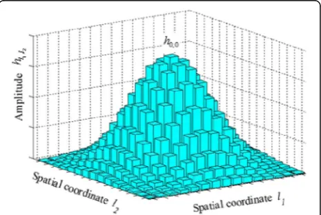
The PSF can be termed as the spatial distribution of optical intensity at the receiving detector for a trans-mitted spatial optical impulse [21, 34]. For the case of an ideal imaging system, the PSF has a distribution of a 2-D Dirac delta function. For the case of a practical imaging system with appropriate focusing, the PSF usually has the distribution of a narrow spatial pulse whose dimensions are mainly a function of the aber-rations of the imaging lens and the diffraction phenomenon at the receiver aperture [11]. In a prac-tical pixelated system, both defocus and motion blur are likely to be present. Defocus is the lack of focus of the imaging lens, while motion blur is caused by the relative motion between the transmitter and the receiver during the exposure time of the imaging sys-tem. These two blurs together cause the received in-tensity pattern to be distributed over a larger space, resulting in a degraded PSF. Figure 4 shows the case of defocus-degraded PSF whose elements can be rep-resented as follows (for simplicity, a 3 × 3 case is shown):
hl1;l2¼
h1;−1 h1;0 h1;1
h0;−1 h0;0 h0;1
h−1;−1 h−1;0 h−1;1
0 @
1
A: ð20Þ
For the case of a stand-alone defocus blur which is often characterized by a 2-D Gaussian (omnidirectional)
SPSF with a spread of σ [28, 35], the elements of (20)
are defined as:
h1;−1¼h−1;−1¼h1;1¼h−1;1 ð21Þ
and
h1;0¼h−1;0¼h0;1¼h0;−1: ð22Þ
On the other hand, it is also difficult to establish a uni-versal model for motion blur since it varies depending on the actual motion during the exposure time of the
(a)
(b)
Fig. 3Illustration of SSFO foram′1¼m′2¼2 and forbm′1¼m′2¼1:5
imaging lens [36]. However, in the literature of
photog-raphy and image processing [37–40], motion blur is
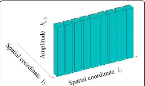
often modelled as simple motion models, e.g. linear con-stant speed motion. Similarly, in this paper, the motion blur is described as a linear motion across a number of pixels in a single (horizontal or vertical) direction and therefore has an APSF distribution. This is illustrated in Fig. 5. It can be seen that the term hl1;l2 for APSF has values only in one dimension and obviously does not fol-low the relationship shown in (21) and (22).
For the case of combined defocus and motion blur, the composite PSF is also asymmetric since it is the convo-lution of the defocus-degraded PSF and the motion-degraded PSF.
5 Simulation results
In this section, the system performance for SACO-OFDM and NCS-SACO-OFDM are evaluated via computer simulations using MATLAB software. In a practical scenario, the numbers of total subcarriers, transmitter/ receiver pixels and the magnitudes of channel impair-ments can vary to a large extent; therefore, there is no standard single value for the simulation parameters. For this paper, the parameters used in the simulations were 256 × 256 subcarriers having a CP and a CPo of 10 % (rounded up to the next integer) each. Moreover, the level of defocus was set as a spread of 9 × 9 SPSF
with σ= 0.5. The motion blur was modelled as a
lin-ear motion across Nd pixels in the horizontal
direc-tion, where Nd= 1, 2 and 4. The combination of the
defocus blur and the motion blur was used to simulate the effect of APSF. Next, the effect of SSFO was simulated for m′= 1.5, 2.5 and 3.5, where m′¼m′1¼m′2. For the case of equalization, a single-step spatial-frequency domain equalizer was used. When the higher subcarriers were not used for data transmission, the number of unused higher spatial-frequency index subcarriers in each dimension,Nh,
was set equal to N/2 where N1=N2=N. In the
simula-tions, the effects of temporal distortions were ignored. Figure 6 shows the constellation diagrams of the trans-mitted and the received SACO-OFDM signals. For Figs. 6a, b, the effect of AWGN is ignored to focus on other impairments. Moreover, for clarity only 64 × 64 subcarriers are used. Figure 6a illustrates the received
constellation points for the case of APSF with Nd= 2
andσ= 0.5 as well as for the case of SPSF withσ= 0.5. It can be seen that the effect of SPSF is only to cause tenuation in the spatial-frequency domain, and the at-tenuation varies depending on the spatial-frequency index. On the other hand, the effect of APSF is to create both attenuation and phase distortions in the spatial-frequency domain. It is clear that the constellation points experience more spread due to APSF than SPSF. Figure 6b presents the received signal for the case of
SSFO wherem′= 1.5. It can be seen that because of the
presence of SSFO, the received constellation points experience attenuation as well as phase distortions.
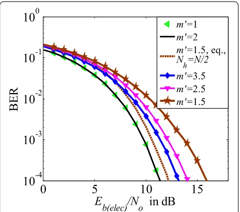
Figure 7 presents the BER as a function ofEb(elec)/N0,
the received electrical energy per bit to single-sided noise spectral density, for the case of stand-alone AWGN and SSFO with and without equalization. In this case, the Eb(elec)/N0 penalty caused by a particular
im-pairment is calculated, at a BER of 10−4, as the Eb(elec)/
N0 difference between the plot for that impairment
(added with AWGN) and the plot for a stand-alone
AWGN system indicated by m′= 1. Note that as
men-tioned in Section 4.1, there is no extra degradation due
to SSFO when m′has any integer value of 2. It can be
seen that the Eb(elec)/N0penalty due to SSFO is
approxi-mately 4.5, 2.8 and 2 dB form′= 1.5,m′= 2.5 andm′= 3.5, respectively, when there is no equalization. This is because as shown in Section 4.1 the larger the values of m′1 andm′2, the less is the spatial-averaging effect, so the less the power penalty. Hence, the receiver should have more number of pixels than the transmitter to combat the effect of SSFO. It can also be seen from
Fig. 7 that the degradation due to SSFO can be
fur-ther reduced when an equalizer is used and the higher subcarriers are not used to carry the data. However, the unused subcarriers reduce the effective data transmission rate.
Figure 8 presents the BER as a function of Eb(elec)/N0,
for the case of stand-alone AWGN, SPSF and APSF. All these plots are for the case of equalization with only lower subcarriers carrying data, i.e.Nh=N/2. It can be seen that
the Eb(elec)/N0 penalties due to SPSF with Nd= 0, APSF
withNd= 1,Nd= 2 andNd= 4 are approximately 2, 2.7, 7
and 10 dB respectively. So, the BER degradation is greater for the case of APSF than for SPSF and for greater values ofNd. This is because as shown earlier, the APSF
addition-ally causes phase distortions which is absent in the case of
SPSF and the level of asymmetry in APSF distribution
in-creases with the increase of Nd. So when motion blur
takes place across a greater number of pixels, the BER degradation becomes more prominent.
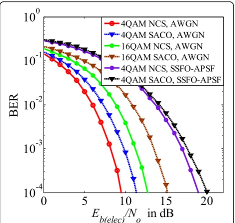
Figure 9 presents the BER as a function ofEb(elec)/N0,
for SACO-OFDM and NCS-OFDM. It can be seen that for AWGN-only channels and for a given constellation size of 4-QAM, NCS-OFDM is 2.0 dB better than SACO-OFDM, but the difference increases to 2.7 dB for 16-QAM. This is because for a given power level, larger constellation points are more susceptible to noise and thus cancelling the noise results in more BER im-provement. Note that the improvement of 2.7 dB due to noise cancellation is close to the 3-dB improve-ment as improve-mentioned for an ideal case in Section 3.2. It can also be seen that for the joint case of SSFO with
m′= 1.5, APSF with Nd= 2 and σ= 0.5 as well as
AWGN, 4-QAM NCS-OFDM is only 1 dB better than 4-QAM SACO-OFDM. So the performance dif-ference between NCS-OFDM and SACO-OFDM is
re-duced in SSFO-APSF channels than stand-alone
AWGN channels. Thus, the effectiveness of noise cancellation in NCS-OFDM is dropped when the im-pairments of SSFO and APSF exist. By comparing the curves for 4-QAM NCS-OFDM in AWGN and SSFO-APSF channels, it can be seen that there can be as large as 8.5 dB degradation in NCS-OFDM due to a given value of SSFO and APSF.
In the following, the BER performance of NCS-OFDM will be compared with that of SACO-OFDM and SDCO-OFDM in terms of average optical power. Since SACO-OFDM/NCS-OFDM uses half the subcarriers of
Fig. 7BER versusEb(elec)/N0for the case of SSFO. Here,eq.stands for
equalization andNhindicates the unused higher subcarriers Fig. 8BER versusEb(elec)/N0for stand-alone AWGN, SPSF and APSF
(a)
(b)
SDCO-OFDM [26], SACO-OFDM/NCS-OFDM with 16-QAM and 256-QAM should be compared with SDCO-OFDM with 4-QAM and 16-QAM, respect-ively. In a recent study [29], it has been shown that
for an optimal bias of 0.80σx, SDCO-OFDM with
4-QAM shows better optical power efficiency than
SACO-OFDM with 16-QAM for Nh=N/2 and for
equalization, where σx is the standard deviation of
xl1;l2. The result reported in [29] is for a given value of vignetting and fractional misalignment and SPSF/
defocus with a spread of σ= 0.5. Figure 10 presents
the BER as a function of Eb(opt)/N0, the received
op-tical energy per bit to single-sided noise spectral density, for NCS-OFDM, SACO-OFDM and SDCO-OFDM with an optimal bias of 0.80σx. In this case, the values of vignetting and fractional misalignment are the
same as those reported in [29]; SSFO is for m′= 1.5,
while APSF is for σ= 0.5 and Nd= 2. Figure 10 shows
that for a given data rate, for Nh=N/2 and for
equalization, 16-QAM NCS-OFDM shows better per-formance than 16-QAM SACO-OFDM and 4-QAM SDCO-OFDM. By comparing the curves for NCS-OFDM in the presence of stand-alone AWGN and all impairments, it is clear that the Eb(opt)/N0 penalty due
to a given value of vignetting, fractional misalignment error, SSFO and APSF is approximately 14 dB.
6 Conclusions
This paper shows that SSFO and motion blur can impair the BER performance of spatial OFDM based
communication systems. The individual presence of SSFO and the simultaneous presence of defocus and
motion blur modelled together as APSF cause
attenuation and phase distortion in the spatial-frequency domain. However, the effect of SSFO can be decreased by ensuring that the number of re-ceived pixels is much larger than the transmitted pixels. Moreover, the use of an equalizer and the use of only the lower subcarriers can further minimize the effect of SSFO. The effect of APSF is different from that of SPSF since SPSF does not cause phase distortion. Depending on the magnitude of motion blur, APSF can create significant BER degradations even when the higher subcarriers are unused for data transmission. Therefore, the relative motion be-tween the transmitter and the receiver must be kept to minimum to ensure reliable data transmission. Next, it is shown that the performance of SACO-OFDM in the joint presence of SSFO and APSF can be improved by forming NCS-OFDM by exploiting the anti-symmetry property of SACO-OFDM. Simu-lation results show that for a given data rate and for the combined perturbations of vignetting, fractional misalignment, SSFO and APSF, NCS-OFDM shows slightly better optical power efficiency than SACO-OFDM
and SDCO-OFDM. Since the above-mentioned
impairments can cause Eb(opt)/N0 penalty as large as
14 dB, efficient techniques will be required to realize practical compensation of these distortions in a
physical system for specific target performance
levels.
Fig. 10BER versusEb(opt)/N0for 16-QAM SACO-OFDM, 4-QAM
SDCO-OFDM and 16-QAM NCS-OFDM.All Impindicates the combined impairments of vignetting, misalignment, SSFO, APSF and AWGN
Fig. 9BER versusEb(elec)/N0 for NCS-OFDM and SACO-OFDM
Competing interests
The author declares that he has no competing interests.
Received: 28 September 2015 Accepted: 24 September 2016
References
1. D Borah, A Boucouvalas, C Davis, S Hranilovic, K Yiannopoulos, A review of communication-oriented optical wireless systems. EURASIP J. Wirel. Commun. Netw.2012(1), 91 (2012)
2. K Langer, J Grubor, Recent developments in optical wireless communications using infrared and visible light, inInternational Conference on Transparent Optical Networks (ICTON), Rome, Italy, 2007
3. D O’Brien, M Katz, P Wang, K Kalliojarvi, S Arnon, M Matsumoto et al., Short-range optical wireless communications, inTechnologies for the Wireless Future: Wireless World Research Forum (WWRF), 2006, p. 2 4. S Rodriguez Perez, B Rodriguez Mendoza, R Perez Jimenez, O Gonzalez
Hernandez, A Garcia-Viera Fernandez, Design considerations of conventional angle diversity receivers for indoor optical wireless communications. EURASIP J. Wirel. Commun. Netw.2013(1), 221 (2013)
5. RJ Green, H Joshi, MD Higgins, MS Leeson, Recent developments in indoor optical wireless systems. IET Commun.2(1), 3–10 (2008)
6. J-B Wang, X-X Xie, Y Jiao, M Chen, Training sequence based frequency-domain channel estimation for indoor diffuse wireless optical communications. EURASIP J. Wirel. Commun. Netw.2012(1), 326 (2012) 7. D O’Brien, R Turnbull, HL Minh, G Faulkner, O Bouchet, P Porcon et al.,
High-speed optical wireless demonstrators: conclusions and future directions. J. Lightw. Technol.30(13), 2181–2187 (2012)
8. L Zeng, D O’Brien, H Minh, G Faulkner, K Lee, D Jung et al., High data rate multiple input multiple output (MIMO) optical wireless communications using white LED lighting. IEEE J. Sel. Areas Commun.27(9), 1654–1662 (2009)
9. S Arnon, Optimised optical wireless car-to-traffic-light communication. Transactions on Emerging Telecommunications Technologies25(6), 660–665 (2014)
10. B Ghimire, H Haas, Self-organising interference coordination in optical wireless networks. EURASIP J. Wirel. Commun. Netw.2012(1), 131 (2012) 11. S Hranilovic, FR Kschischang, A pixelated MIMO wireless optical communication
system. IEEE J. Sel. Topics Quantum Electron.12(4), 859–874 (2006) 12. HBC Wook, T Komine, S Haruyama, M Nakagawa, Visible light
communication with LED-based traffic lights using 2-dimensional image sensor, inIEEE Consumer Communications and Networking Conference (CCNC), 2006
13. A Ashok, M Gruteser, NB Mandayam, J Silva, M Varga, KJ Dana, Challenge: mobile optical networks through visual MIMO, inInternational Conference on Mobile Computing and Networking (MobiCom), Chicago, Illinois, USA, 2010 14. SD Perli, N Ahmed, D Katabi, PixNet: interference-free wireless links using
LCD-camera pairs, inInternational Conference on Mobile Computing and Networking (MobiCom), Chicago, Illinois, USA, 2010
15. T Hao, R Zhou, G Xing, COBRA: color barcode streaming for smartphone systems, inInternational Conference on Mobile Systems, Applications and Services (MobiSys), Lake District, UK, 2012
16. S Kuzdeba, AM Wyglinski, B Hombs,Prototype Implementation of a Visual Communication System Employing Video Imagery, presented at the IEEE Consumer Communications and Networking Conference (CCNC), Las Vegas, NV, USA (11–14 Jan), 2013
17. S Arai, S Mase, T Yamazato, T Yendo, T Fujii, M Tanimoto et al.,Feasible Study of Road-to-Vehicle Communication System Using LED Array and High-Speed Camera, presented at the 15th World Congress on ITS, USA, 2008
18. MRH Mondal, J Armstrong, Analysis of the effect of vignetting on MIMO optical wireless systems using spatial OFDM. J. Lightw. Technol.32(5), 922–929 (2014)
19. W Yuan, K Dana, M Varga, A Ashok, M Gruteser, N Mandayam, Computer vision methods for visual MIMO optical system, inIEEE Computer Society Conference on Computer Vision and Pattern Recognition Workshops (CVPRW), Colorado, USA, 2011, pp. 37–43
20. MDA Mohamed, S Hranilovic, Two-dimensional binary halftoned optical intensity channels. IET Communications, Special Issue on Optical Wireless Communication Systems2(1), 11–17 (2008)
21. A Dabbo, S Hranilovic, Receiver design for wireless optical MIMO channels with magnification, in10th International Conference on Telecommunications, Zagreb, Croatia, 2009
22. C Pei, Z Zhang, S Zhang,SoftOC: Real-Time Projector-Wall-Camera Communication System, presented at the IEEE International Conference on Consumer Electronics (ICCE), Las Vegas, NV, USA, 2013
23. LL Hanzo, Y Akhtman, L Wang, M Jiang,MIMO-OFDM for LTE, WiFi and WiMAX: Coherent versus Non-Coherent And Cooperative Turbo Transceivers (John Wiley & Sons Ltd., Oct. 2010)
24. MRH Mondal, SP Majumder. Analytical performance evaluation of space time coded MIMO OFDM systems impaired by fading and timing jitter, Journal of Communications.4(6) (2009)
25. A Loulou, M Renfors, Enhanced OFDM for fragmented spectrum use in 5G systems. Transactions on Emerging Telecommunications Technologies 26(1), 31–45 (2015)
26. MRH Mondal, KR Panta, J Armstrong, Performance of two dimensional asymmetrically clipped optical OFDM, in2010 IEEE Globecom Workshops (GC’10), Piscataway, NJ, USA, 2010
27. MRH Mondal, J Armstrong, Impact of linear misalignment on a spatial OFDM based pixelated system, inAsia Pacific Conference on Communications (APCC), Jeju Island, South Korea, 2012
28. MRH Mondal, J Armstrong, The effect of defocus blur on a spatial OFDM optical wireless communication system, in14th International Conference on Transparent Optical Networks (ICTON), Coventry, England, UK, 2012 29. MRH Mondal, K Panta,Performance Analysis of Spatial OFDM for Pixelated
Optical Wireless Systems, Transactions on Emerging Telecommunications Technologies (ETT), 2015
30. Q Pu, W Hu,Smooth Transmission over Unsynchronized VLC links, presented at the International Conference on Emerging Networking Experiments and Technologies (CoNEXT) Student Workshop Nice, France, 2012
31. J Armstrong, AJ Lowery, Power efficient optical OFDM. Electron. Lett.42(6), 370–372 (2006)
32. SK Wilson, J Armstrong,Digital Modulation Techniques for Optical Asymmetrically-Clipped OFDM, presented at the in Proceedings IEEE WCNC, Las Vegas, USA, 2008
33. K Asadzadeh, A Dabbo, S Hranilovic, Receiver design for asymmetrically clipped optical OFDM, inGLOBECOM Workshops (GC Wkshps), 2011 IEEE, 2011, pp. 777–781
34. S Hranilovic, FR Kschischang, Short-range wireless optical communication using pixelated transmitters and imaging receivers, inIEEE Int. Conf. Commun, 2004, pp. 891–895
35. MDA Mohamed, A Dabbo, S Hranilovic, MIMO optical wireless channels using halftoning, inIEEE International Conference on Communications 2008, Beijing, China, 2008
36. M Tico, M Vehvilainen, Estimation of motion blur point spread function from differently exposed image frames, inSignal Processing Conference, 2006 14th European, 2006, pp. 1–4
37. TF Chan, W Chiu-Kwong, Total variation blind deconvolution. IEEE Trans. Image Process.7(3), 370–375 (1998)
38. YL You, M Kaveh, A regularization approach to joint blur identification and image restoration. IEEE Trans. Image Process.5(3), 416–428 (1996) 39. A Agrawal, X Yi, Coded exposure deblurring: optimized codes for PSF
estimation and invertibility, inComputer Vision And Pattern Recognition, 2009. CVPR 2009. IEEE Conference on, 2009, pp. 2066–2073