R E S E A R C H
Open Access
Calibration of the exponential
Ornstein–Uhlenbeck process when spot
prices are visible through the maximum
log-likelihood method. Example with gold
prices
Carlos Armando Mejía Vega
1**Correspondence:
[email protected] 1Externado University of Colombia,
Bogota, Colombia
Abstract
The purpose of this paper is to present a methodological procedure to estimate the parameters of the exponential Ornstein–Uhlenbeck process, also known as the
Schwartz (J. Finance 52(3):923–973,1997) one-factor model, in situations where the
spot price of the commodity is observable. The proposal consists of looking at the probability function of the process as a function of the unknown parameters in discrete time, known as the likelihood function. Then the logarithm of that expression is calculated as it is easier to work with it. Finally, the problem of determining the values of the parameters that maximize the sum of the individual log-likelihoods (joint log-likelihood function) is solved to obtain the estimation equations explicitly. In that sense, this work is relevant because as spot prices are available, it is possible to estimate the parameters directly without the necessity of using more elaborate approaches like the Kalman filter. Finally, the paper applies this methodology to the concrete case of one precious metal that has an observable spot price and for which some empirical and theoretical studies suggest that it presents a mean-reverting pattern, gold. The estimated parameters are consistent with previous works and with the original data and the least squares method.
JEL Classification: C100; C130; G100; G170
Keywords: Commodities; Commodity modelling; Stochastic process; Exponential Ornstein–Uhlenbeck process; Maximum log-likelihood method; Parameters estimation
1 Introduction
Commodities are the essential blocks of humanity, as they are raw materials that are funda-mental to both the sustainability and development of any civilization. Furthermore, many countries specialize in their exportation in international physical markets, which implies that any movement in commodity prices can have significant consequences for them [11]. Finally, in recent years, global commodity financial markets have been rapidly expanding, and commodity futures are nowadays essential assets in any investor portfolio around
the world [32]. Considering all these facts, commodity price analysis and modeling have turned into relevant fields nowadays.
One of the main distinguishing features of most commodity prices against other as-set prices is the presence of a mean-reverting behavior (see, e.g., Bessembinder et al. [4], Casassus and Collin-Dufresne [7], Pyndick [21], Routledge et al. [25], and Schwartz [27], among others, for empirical evidence justifying the usage of mean-reversion for commod-ity prices). Based on this, commodcommod-ity modeling has been applying models with this prop-erty since long time ago [1]. In that sense, the most basic and simplified stochastic process that describes the characteristic of the process to drift toward a long-term value is known as the Ornstein–Uhlenbeck process [8]. It was first used in commodity modeling by Gib-son and Schwartz [12] to model the light sweet (WTI) crude oil net spot instantaneous convenience yield under the umbrella of the storage theory (see Lautier [18] for a complete survey of the storage theory till the models of Schwartz [27]).
The Ornstein–Uhlenbeck process (also known as the arithmetic Ornstein–Uhlenbeck process) is a stochastic process initially proposed by the physicists Leonard Solomon Ornstein and the physicist George Eugene Uhlenbeck in a paper titledOn the theory of the Brownian motion[33]. This work appeared in volume 36 of thePhysical Reviewin September 1930. In general terms, and under a filtered probability space [,F, (Ft≥0),P], a stochastic process{X(t);t≥0}is said to follow an arithmetic Ornstein–Uhlenbeck pro-cess if it satisfies the following stochastic differential equation [19]:
dX(t) =θμ–X(t)dt+σdW(t), (1) wheredX(t) is an increment of the processXbetweentanddt, andσ > 0 is the instan-taneous diffusion term, used to measure the volatility of the process, which is assumed to be constant. On the other side,μis the process long-term expected value, andθ> 0 is the speed or reversion ofX(t) towardμ, both also assumed to be constant. Finally,dW(t) is an increment during the interval (t,t+dt) of a standard Brownian motion under the real probability measureP, which follows a normal distribution with expected value 0 and variancet.
maximum log-likelihood [34], and jackknife technique [20]. Based on this, Chaiyapo and Phewchean [8] calibrated their model with the three methods, whereas Tanaka and Car-rasco Montero [31] used only the least squares method, and Barlow [1] the log-likelihood one. However, even if the parameters were consistent, one of the general limitations is that in all these cases, spot prices can have negative values.
By considering this, and inspired by Ross [24] and Bessembinder et al. [4], the engi-neer Eduardo Schwartz proposed a modification of the geometric Ornstein–Uhlenbeck developed previously by Dixit and Pyndick [10] in a paper titledThe stochastic behav-ior of commodity prices: Implications for valuation and hedging. This model, known as the Schwartz [27] reduced-form, equilibrium one-factor model or as the exponential Ornstein–Uhlenbeck process [3], appeared in volume 52 ofThe Journal of Financein July 1997. In general terms, and under a filtered probability space [,F, (Ft≥0),P], a stochas-tic process{X(t);t≥0}is said to follow an exponential Ornstein–Uhlenbeck process if it satisfies the following stochastic differential equation [27]:
dX(t) =θμˆ–LnX(t)X(t)dt+σX(t)dW(t), (2)
wheredX(t) is an increment of the processXbetweentandt+dt,μˆ andθ > 0 are two constants that affect the instantaneous drift component of the process, anddtis an in-finitesimal increment in time. On the other side,σ> 0 is a third constant that affects the instantaneous diffusion component of the process. Finally,dW(t) is an increment, during the interval (t,t+dt), of a standard Brownian motion under the real probability measure P, which follows a normal distribution with expected value 0 and variancet.
This model has also been used to describe and simulate the general mean-reverting dynamic over time of several commodities spot prices again under the umbrella of the reduced-form one-factor models. In fact, Schwartz [27] applied it for WTI crude oil and for gold and copper. A more recent work of Bastian-Pinto et al. [2] used the same stochas-tic process to model alternative fuels in Brazil into the real options framework. Explicitly, they modeled two types of agricultural commodities (sugar and ethanol). Finally, Brajkovic [6] used this model (as well as the geometric Brownian motion, arithmetic Ornstein– Uhlenbeck process, and Cox–Ingersoll–Ross process) for modeling coal prices and valued a baseload coal-fired power plant under the same real options approach.
With this second model, to make forecasts again, it was also essential to calibrate the model. However, by recognizing the fact that spot prices are not visible (mostly in inter-national commodity markets), Schwartz [27] decided to calibrate the model by relating the spot price with futures prices (which are visible) and then applying a filtering process known as the Kalman filter (for a detailed discussion of the state space models and the Kalman filter, see Harvey [13]) combined with the maximization of a defined joint log-likelihood function. This method is known as the expectation maximization algorithm or the prediction error decomposition (see Harville [14]). Since then, it is the standard procedure to estimate the parameters of this model (see, e.g., Kellerhals [15]).
it could be possible to estimate the parameters by more suitable and tractable methods like the ones mentioned before for the traditional arithmetic Ornstein–Uhlenbeck process. In that sense, Dias [9] applied the least squares method for the exponential Ornstein– Uhlenbeck process and obtained the calibration equations explicitly. However, the cali-bration of this process through the log-likelihood approach has not been entirely devel-oped and analyzed in commodity modeling. In that sense, Brajkovic [6] estimated the pa-rameters of the four models mentioned before to see which ones fit better for coal prices through the joint likelihood function method, but only defined the general problem and used computational ways to solve it in each case.
Based on this, in this paper, we expose a calibration method that does not require the use of filtering processes like the Kalman filter, but only the maximization of a defined joint log-likelihood function. The structure of the paper goes in the following way. In Sect.1, general information about the literature is given. In Sect.2, a general presentation of the stochastic process is provided. In Sect.3, the exposition of the general estimation proce-dure is presented. In Sect.4, the method is applied to gold prices, and finally, in the last section, both the conclusion and discussion for futures works are included.
2 The exponential Ornstein–Uhlenbeck process 2.1 Intuition as a deterministic process
A deterministic process X(t) is said to follow a deterministic exponential Ornstein– Uhlenbeck process if it satisfies the following differential equation:
dX(t) =θμˆ–LnX(t)X(t)dt, (3)
where the drift term depends on the natural logarithm of the current value of the process Ln[X(t)], and the natural logarithm of the long-term expected value of the spot priceμˆ
acts as the equilibrium level of the process:
• If the natural logarithm of the current value of the processLn[X(t)]is lower thanμˆ, then the drift will be positive,θ{ ˆμ–Ln[X(t)]}X(t) > 0anddX(t) > 0.
• If the natural logarithm of the current value of the processLn[X(t)]is higher thanμˆ, then the drift will be negative,θ{ ˆμ–Ln[X(t)]}X(t) < 0anddX(t) < 0.
• This dynamics is known as mean-reverting, whereθ> 0determines the speed of reversion of the process.
2.2 Analytical solution
Considering thatX(t) is an Itô process and applying Itô’s lemma to the functionLn[X(t)]eθt, we get:
dLnX(t)eθt=
θμˆeθt–σ
2eθt 2
dt+σeθtdW(t). (4)
Given equation (4), the integration fromstot, where 0≤s<t, is performed to obtain the analytical solution of equation (2) [27]:
LnX(t)=LnX(s)e–θ(t–s)+
ˆ
μ–σ
2
2θ
1 –e–θ(t–s)+
t
s
2.3 Gaussian property
From equation (5) the expected value and the variance of the processLn[X(t)], conditional to information (Fs)t>s≥0, are given by [27] ditional to information (Fs)t>s≥0, follows the normal distribution (it is a Gaussian process)
with expected valueLn[X(s)]e–θ(t–s)+ (μˆ–σ2
2θ)[1 –e
–θ(t–s)] and varianceσ2
2θ[1 –e
–2θ(t–s)]. The
conditional probability distribution function ofLn[X(t)] under the exponential Ornstein– Uhlenbeck process is given by
fLnX(t)|θ,μˆ,σ
3 Parameters estimation through the maximum log-likelihood method 3.1 Discretization process
Given the availability of an information setFt–1 and an observation interval [0,T], the
exact analytical solution of the exponential Ornstein–Uhlenbeck process in equation (5) can be discretized over a partition with constant intervalt=stepsT in the following way:
Ln(Xt) =Ln(Xt–1)e–θ t+
whereεtis an error driven by the normal distribution with expected value 0 and variance 1. In that sense, the processLn(Xt), conditional to informationFt–1, follows the normal
distribution with expected valueLn(Xt–1)e–θ t+ (μˆ–σ
where ηt is an error driven by the normal distribution with expected value 0 and vari-anceσ2θ2(1 –e–2θ t). The processLn(X
t), conditional to informationFt–1, again follows the
normal distribution with expected valueLn(Xt–1)e–θ t+ (μˆ–σ
3.2 The joint log-likelihood function
and (9) or (10), the likelihood function is given by [23]
However, for practical purposes, it is better to use the log-likelihood function given by
LnLθ,μˆ,σ|Ln(Xt) hood function is given by
n
The next step consists in taking the partial derivatives and equal them to zero. In that sense, the partial derivative with respect toμˆˆ is taken:
Considering equation (12), we then have:
ˆ
μ=μˆˆ+σ
2
2θ. (20)
Next, the partial derivative with respect toθ is taken:
∂ni=1Ln{L[θ,μˆ,σ|Ln(Xi)]}
Finally, the partial derivative with respect toσˆ is taken:
Considering equation (13), we then have:
One of the problems with the last solutions is that each parameter depends on each other. However, by replacingθ intoμˆˆthis can be solved:
ˆˆ
Considering this, all the parameters can be obtained through the following steps: • Obtainμˆˆ from (30), (31), and (32).
• Then obtainθ from (24). • Then obtainσˆ2from (28).
• Then obtainσ2from (29). • Finally, obtainμˆ from (20).
4 Results for gold and discussion 4.1 Gold spot prices
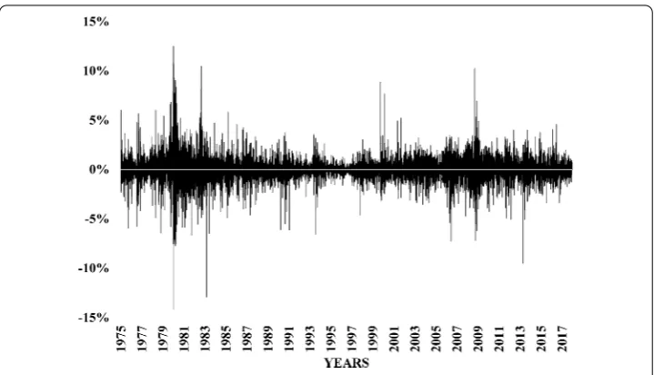
The Bretton Woods Conference (also known as the United Nations Monetary and Finan-cial Conference) established a permanent exchange rate between one troy ounce of gold and the United States dollar. In 1972 the fixed rate system ended, but the logic of an ex-change rate between the precious metal and the currency persisted in what is now known as the XAUUSD in Foreign Exchange Markets (FOREX). This exchange rate acts as a spot price for gold [29]. Daily gold spot prices from January 02, 1975, to December 29, 2017, are shown in Fig.1. These data were taken from Bloomberg. On the other side, the nat-ural logarithm and the logarithm returns of this series are exhibited in Fig.2and Fig.3, respectively.
The descriptive statistics of the gold spot price, its natural logarithm, and the logarithm returns both daily and annually (by taking the annual average) are exhibited in Table1
Figure 1Daily gold spot price from January 02, 1975, to December 29, 2017.Source of data: Bloomberg XAUUSD Currency
Figure 2Natural logarithm of the daily gold spot price from January 02, 1975, to December 29, 2017.Source of data: Bloomberg XAUUSD Currency
4.2 Calibration process
Figure 3Daily logarithm returns of the gold spot price from January 02, 1975 to December 29, 2017.Source of data: Bloomberg XAUUSD Currency
Table 1 Descriptive statistics of the daily gold spot price, its natural logarithm, and its logarithm returns.Source: Data from Bloomberg XAUUSD
Daily Standard Spot Price Natural Logarithm Logarithm return
Mean 577.27 6.14 0.02%
Standard deviation 416.02 0.65 1.23%
Skewness 1.30 0.38 0.02
Kurtosis 3.46 2.56 14.45
Table 2 Descriptive statistics of the annual gold spot price, its natural logarithm, and its logarithm returns.Source: Data from Bloomberg XAUUSD
Annual Standard Spot Price Natural Logarithm Logarithm return
Mean 573.70 6.14 4.90%
Standard deviation 415.65 0.65 19.07%
Skewness 1.34 0.41 0.97
Kurtosis 3.56 2.67 5.23
Shafee and Topal [28] found that the first difference of gold spot price was stationary, sug-gesting a mean-reversion pattern. Based on these past studies, it is possible to think that the exponential Ornstein–Uhlenbeck process could be a good model for the gold spot price.
The next step is to calibrate the exponential Ornstein–Uhlenbeck process with the daily data presented in Sect.4.1by takingt= 1 (to obtain daily parameters) applying equations (30), (31), (32), (24), (28), (29), and (20). Then, the same procedure is repeated but now settingt= 1/250 (to obtain annualized parameters). Finally, the calibration is done with the average annual data by taking againt= 1 (to obtain annual parameters). The results are presented in Table3.
Table 3 Parameters of the exponential Ornstein–Uhlenbeck process obtained for the gold spot price through the maximum log-likelihood method
Miu hat Theta Sigma
Daily 7.22 0.0002 1.23%
Annualized 7.67 0.0420 19.42%
Annual 7.49 0.0497 19.06%
changing thetwith little significant errors for the case of gold. Furthermore, some gen-eral conclusions are the following:
• The reversion speedθindicates that the natural logarithm of the gold spot price (and hence the price) reverts to its long-term expected value in around 0.04971 years or 20 years (for the daily and annualized parameters it will be 0.0002∗2501 or 0.04201 years, equal in both cases to almost 24 years). This low speed of reversion is consistent with previous research works like those of Schwartz [27], Bessembinder et al. [4], Shafee and Topal [28], and Tanaka and Carrasco [31].
• On the other side, both the annualized and annual volatilities are of around 19%, which confirms gold as having moderate price volatility, and it is consistent with the historical annual standard deviation of the logarithm returns provided before in Table2, reflecting the consistency of the calibration process again.
4.3 Comparison with the least squares method
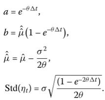
To see if the obtained parameters are not only consistent with previous works and the information itself, they were also estimated through the least squares method developed by Dixit and Pyndick [10] and modified by Dias [9]. However, in this case, the regression was constructed by following equation (10), so that it relates the natural logarithm of the spot price (rather than the logarithm return) with the natural logarithm of the first lag in the same way Van den Berg [34] did for the arithmetic Ornstein–Uhlenbeck process. The regression equation is then given by
Ln(St) =aLn(St–1) +b+ηt, (33)
where
a=e–θ t, (34)
b=μˆˆ1 –e–θ t, (35) ˆˆ
μ=μˆ–σ
2
2θ, (36)
Std(ηt) =σ
(1 –e–2θ t)
2θ . (37)
Rewriting the equations gives
θ= –Ln(a)
t , (38)
ˆˆ
μ= b
Table 4 Coefficients of the exponential Ornstein–Uhlenbeck process obtained for the gold spot price through the least squares method
a b Std(η)
Daily 0.9998 0.0012 1.23%
Annual 0.9515 0.3451 19.06%
Table 5 Parameters of the exponential Ornstein–Uhlenbeck process obtained for the gold spot price
through the least squares method
Miu hat Theta Sigma
Daily 7.22 0.0002 1.23%
Annualized 7.22 0.0420 19.42%
Annual 7.12 0.0497 19.53%
σ=Std(ηt)
–2Ln(a)
t(1 –a2), (40)
ˆ
μ=μˆˆ+σ
2
2θ. (41)
The next step is to calibrate the exponential Ornstein–Uhlenbeck process with the daily data presented in Sect.4.1by takingt= 1 (to obtain daily parameters), by running the regression of equation (33), and finally applying equations (38), (39), (40), and (41). Then, the same procedure is repeated but now settingt= 1/250 (to obtain annualized param-eters). Finally, the calibration is done with the average annual data and by taking again
t= 1 (to obtain annual parameters). The results of the coefficientsaandband of the standard deviation of the error for both daily and annual data are presented in Table4. On the other side, the estimated parameters are shown in Table5.
By looking at Table5it is possible to conclude that the three parameters are similar in daily, annualized, and annual terms, and so the proposed methodology is also consistent with the least squares method.
5 Conclusions
One of the main difficulties in commodity modeling is the estimation of the parameters of the stochastic processes used to model the dynamics over time of both the spot price and other state variables. One of the main reasons for this is the fact that most of these state variables are not observable for many commodities (mainly in international markets). In that sense, the calibration of general processes like the exponential Ornstein–Uhlenbeck process is done through filtering algorithms like the Kalman filter.
Futures works might include restrictions to some of the parameters, as some of them can-not have negative values and the present methodology does can-not impose those conditions. Also, as the maximum log-likelihood method produces a punctual estimator for each pa-rameter, further extensions could be to define intervals for each estimator given a confi-dence level.
Acknowledgements
The author would like to thank the editor and referees for their valuable suggestions, which improved the structure and the presentation of the paper.
Funding
Not applicable.
Competing interests
The author declares having no competing interests.
Authors’ contributions
All authors read and approved the final manuscript.
Publisher’s Note
Springer Nature remains neutral with regard to jurisdictional claims in published maps and institutional affiliations.
Received: 26 March 2018 Accepted: 15 June 2018 References
1. Barlow, M.T.: A diffusion model for electricity prices. Math. Finance12(4), 287–298 (2002)
2. Bastian-Pinto, C., Brandão, L., Hahn, W.J.: Flexibility as a source of value in the production of alternative fuels: the ethanol case. Energy Econ.31(3), 411–422 (2009)
3. Benth, F.E., Karlsen, K.H.: A note on Merton’s portfolio selection problem for the Schwartz mean-reversion model. Stoch. Anal. Appl.23(4), 687–704 (2005)
4. Bessembinder, H., Coughenour, J.F., Seguin, P.J., Smoller, M.M.: Mean reversion in equilibrium asset prices: evidence from the futures term structure. J. Finance50(1), 361–375 (1995)
5. Bona, T., Llansana, J.: Física y Química. Carroggio, Barcelona (1999)
6. Brajkovic, J.: Real-options approach to investment in base load coal fired plant. Working paper (2010) 7. Casassus, J., Collin-Dufresne, P.: Stochastic convenience yield implied from commodity futures and interest rates.
J. Finance60(5), 2283–2331 (2005)
8. Chaiyapo, N., Phewchean, N.: An application of Ornstein–Uhlenbeck process to commodity pricing in Thailand. Adv. Differ. Equ.2017(1), 179 (2017)
9. Dias, M.: Stochastic processes with focus in petroleum applications, Part 2—mean reversion models. http://marcoagd.usuarios.rdc.puc-rio.br/revers.html#mean-rev
10. Dixit, A.K., Pindyck, R.S.: Investment Under Uncertainty. Princeton University Press, Princeton (1994) 11. Geman, H.: Commodities and Commodity Derivatives. Wiley, West Sussex (2005)
12. Gibson, R., Schwartz, E.S.: Stochastic convenience yield and the pricing of oil contingent claims. J. Finance45(3), 959–976 (1990)
13. Harvey, A.C.: Forecasting, Structural Time Series Models and the Kalman Filter. Cambridge University Press, Cambridge (1990)
14. Harville, A.: Decomposition of prediction error. J. Am. Stat. Assoc.80(389), 132–138 (1985)
15. Kellerhals, B.P.: Financial Pricing Models in Continuous Time and Kalman Filtering. Springer, Berlin (2001) 16. Laguna, A.: Modern Supramolecular Gold Chemistry: Gold-Metal Interactions and Applications. Wiley, Weinheim
(2008)
17. Laughton, D.G., Jacoby, H.D.: Reversion, timing options, and long-term decision-making. Financ. Manag.22(3), 225–240 (1993)
18. Lautier, D.: Term structure models of commodity prices: a review. J. Altern. Invest.8(1), 42–64 (2005)
19. Önalan, O.: Financial modelling with Ornstein–Uhlenbeck processes driven by Lévy process. In: Proceedings of the World Congress on Engineering, London (2009)
20. Phillips, P.C.B., Yu, J.: Jackknifing bond option prices. Rev. Financ. Stud.18(2), 707–742 (2005)
21. Pyndick, R.S.: The dynamics of commodity spot and futures markets: a primer. Energy J.22(3), 1–29 (2001) 22. Ribeiro, D.R., Hodges, S.D.: Equilibrium model for commodity prices: competitive and monopolistic markets. Working
Paper (2004)
23. Rohde, C.A.: Introductory Statistical Inference with the Likelihood Function. Springer, New York (2014) 24. Ross, S.: Hedging long run commitments: exercises in incomplete market pricing. Working paper (1995)
25. Routledge, B.R., Seppi, D.J., Spatt, C.S.: Equilibrium forward curves for commodities. J. Finance55(3), 1297–1338 (2000) 26. Sauvageau, M., Kumral, M.: Genetic algorithms for the optimization of the Schwartz–Smith two-factor model: a case
study on a copper deposit. Int. J. Surf. Min. Reclam. Environ.32(3), 163–181 (2018)
28. Shafiee, S., Topal, E.: An overview of global gold market and gold price forecasting. Resour. Policy35(3), 178–189 (2010)
29. Sjaastad, L.A.: The price of gold and the exchange rates: once again. Resour. Policy33(2), 118–124 (2008)
30. Smith, W.: On the simulation and estimation of mean-reverting Ornstein–Uhlenbeck process: especially as applied to commodities markets and modelling (2010)
31. Tanaka, A.T., Carrasco, C.M.: Valorización de opciones reales: el modelo Ornstein–Uhlenbeck. J. Econ. Finance Adm. Sci.21(41), 56–62 (2017)
32. Tang, K., Wei, X.: Index investment and the financialization of commodities. Financ. Anal. J.68(5), 54–74 (2012) 33. Uhlenbeck, G.E., Ornstein, L.S.: On the theory of the Brownian motion. Phys. Rev.36, 823–841 (1930) 34. Van den Berg: Calibrating the Ornstein–Uhlenbeck (Vasicek) model.