Distributed and Collaborative Node Mobility Management for Dynamic Coverage Improvement in Hybrid Sensor Networks

Volume 2011, Article ID 724136,17pages doi:10.1155/2011/724136

Research Article

Distributed and Collaborative Node Mobility Management for

Dynamic Coverage Improvement in Hybrid Sensor Networks

Thakshila Wimalajeewa

_{and Sudharman K. Jayaweera}

1_{Department of Electrical Engineering and Computer Science, Syracuse University, Syracuse, NY 13244, USA} 2_{Department of Electrical and Computer Engineering, University of New Mexico, Albuquerque, NM 87131, USA}

Correspondence should be addressed to Thakshila Wimalajeewa,[email protected]

Received 25 April 2010; Revised 15 January 2011; Accepted 4 February 2011

Academic Editor: Amiya Nayak

Copyright © 2011 T. Wimalajeewa and S. K. Jayaweera. This is an open access article distributed under the Creative Commons Attribution License, which permits unrestricted use, distribution, and reproduction in any medium, provided the original work is properly cited.

With recent advances in deploying sensor nodes mounted on mobile platforms, node mobility is becoming an attractive alternative

to improve network coverage dynamically in sensor networks. However, due to energy constraints, it may not be cost effective to

deploy a large number of mobile nodes for continuous movements. It might be more desirable to allow only a certain number of

nodes to be mobile depending on the affordable cost and desired performance levels. This paper proposes an efficient distributed

mobility protocol for mobile node navigation in a hybrid sensor network consisting of both static and mobile nodes to provide

efficient time-varying coverage after the initial deployment. In the proposed scheme, mobile nodes collaborate with neighboring

static nodes to find their candidate locations to move at each movement step in order to maximize thecoverage timeof the area not

covered by static nodes. We also develop an efficient sequential algorithm to find theexposurein a hybrid network, which reflects

the best path for a target to traverse the sensing region without being detected. By simulations, we show the effectiveness of the

proposed mobility protocol in terms of the presence probability matrix andcoverage timeand show its suitability at the worst-case

targetexposure.

1. Introduction

Mobile sensor nodes are deployed in wireless sensor net-works in certain applications to enhance the network per-formance dynamically. Use of node mobility to reposition sensors at the deployment stage to provide a uniform cov-erage was considered in [1–5], based on different techniques. However, these studies do not consider how to exploit the node mobility in possible performance improvement after the initial deployment stage. Liu et al. in [6] showed that the coverage can be improved dynamically by allowing nodes to be mobile continuously in a mobile sensor network over time unlike in a static network. Distributed detection and tracking tasks by mobile sensor networks consisting only mobile nodes were addressed by some recent work. In [7], the problem of target detection using a mobile sensor network is addressed where the authors analyzed the detection latency. In [8], algorithms to find upper and lower bounds for the targetexposure, which is defined as the target traversal which

at the initial deployment stage are developed in hybrid sensor networks. In [12], mobile nodes are directed to move towards the coverage holes detected by static nodes to improve the coverage. In [13], impact of the node density to providek -coverage at the deployment stage in a hybrid sensor network is discussed. In these approaches, it was assumed that the mobile nodes move only once during the deployment stage and remain stationary while the sensor network performs specific operations. In [14], mobile node navigation towards a specific goal in a hybrid sensor network is addressed where static nodes are used to guide the mobile nodes. Distributed detection by hybrid sensor networks is also addressed in recent works [15, 16] when the sensor node and target positions are known. Target tracking performance of an integrated mobile-static sensor network is addressed in [17] where the mobile nodes are used to aid the data propagation when the communication ranges of static nodes are limited. However, neither of the above works addressed the problem of how to efficiently cover the uncovered area by static nodes in a hybrid sensor network dynamically, by node mobility over time to provide an efficient time-varying coverage.

2. Motivation, Contribution,

and Organization

Consider a hybrid sensor network deployed in a square region as shown in Figure 1, where the union of checked circles represents the area covered by static nodes while the union of solid circles represents the area covered by mobile nodes, respectively. When the nodes are first deployed in a region, a random placement is often desirable especially

when a priori knowledge of the terrain is unavailable.

However, such random deployment strategies may not result in effective coverage always, since some nodes might be overly clustered while some of them might be sparsely located. Use of node mobility to reconfigure the node locations to improve the coverage of such networks was addressed by some authors, for example, in [1,2,12]. In these approaches, nodes move only during the deployment stage and the maximum coverage area achieved by the network after reconfiguration is limited by the number of total nodes and nodes’ sensing ranges. For example, if the total number of nodes is relatively small, even by reconfiguration of mobile nodes to provide a uniform coverage, a large portion of the network may remain not covered. On the other hand, node failures after the initial reconfiguration might cause coverage holes in the network. Thus, the problem addressed in this paper is how to effectively use the node mobility of mobile nodes to provide an efficient dynamic coverage of the region of interest after the initial deployment stage.

Exploiting mobile nodes for continuous coverage in mobile sensor networks is addressed by [6] when the nodes perform random and independent mobility. Although random mobility models are desirable in many applications, and they need minimum coordinations among nodes, they may not always be ideal for hybrid networks consisting of both static and mobile nodes. We need to consider the following factors in designing an algorithm for mobile node

Figure 1: Hybrid sensor network consisting of both static and mobile nodes: solid circles-mobile nodes and checked circles-static nodes.

navigation in a hybrid sensor network to provide efficient dynamic coverage.

(i) In a hybrid sensor network, a certain portion of the field is covered always (as shown by the union of checked circles in Figure 1) as mentioned before. Mobile nodes are required to assist providing the coverage for the area that is not covered by static nodes. If a random and independent mobility scheme is used, there might be overlappings of the sensing ranges of mobile and static nodes since there is no coordination among nodes. In many real world applications, a mobile node (a sensor node mounted on a mobile platform,) has a fixed power cost for the mobility. Even though sensor nodes mounted on mobile platforms can carry more battery supplies to move a considerable amount of time/distance continuously, it is important to ensure that the available energy is effectively used to perform the required surveillance task, that is, to provide an effective time-varying coverage in the desired field in a given duration of time. Thus, it is required to use mobile nodes to cover only the areas uncovered by static nodes minimizing the overlapping between the mobile and static nodes’ sensing ranges.

(ii) When nodes are mobile, previously covered areas by mobile nodes become uncovered while uncovered areas become covered. This requires to manage the mobility of the mobile nodes such that to minimize the duration that a particular location is uncovered. Random mobility schemes do not address these issues.

(iii) If the network does not have any prior knowledge about the sensing field, it is desired that any point not covered by the static nodes is covered almost equally to maintain an approximately uniform coverage over time.

scheme, collaborating with static nodes, mobile nodes pro-vide an efficient dynamic coverage in the area not covered by the static nodes. More specifically, we assume that the sensor network is partitioned into square cells such that a node can cover such a cell completely when it is located at the center of the cell. We divide these cells into two categories:staticand

voidcells.Staticcells correspond to the cells in which there is at least one static node, and thevoidcells are the ones in which there is no any static node. Mobile nodes are directed to move among thesevoidcells based on a certain criteria. Each of suchvoidcells is given a certainbase price. Thisbase priceis updated by static nodes based on the time that the

voidcell remains not covered by at least one mobile node. At each movement step, mobile nodes communicate with their closest static nodes locally to search forvoidcells which are not covered for a long time. Static nodes provide necessary information for mobile nodes in their neighborhoods. At a given time, we assume that a mobile node can visit a certain number of candidate void cells from its current position. These candidate voidcells are determined by the mobile node’s maximum speed. Taking base prices (collected from neighboring static nodes) of the candidate voidcells into account, each mobile node selects the best voidcell to be visited by the next time step. In the proposed scheme, since the node mobility is performed by mobile nodes by collaborating with static nodes, we call the proposed scheme “mobile-static collaborative mobility model.” In simulations, we show the effectiveness of the mobile-static collaborative mobility modelin terms of the presence probability matrix and the average time that an arbitrary point in the network is not covered. (The presence probability matrix contains the probabilities of the presence of at least one node at each cell at any given time instant.)

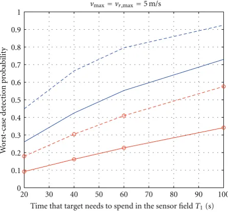
We further analyze the effectiveness of the proposed mobility scheme in terms of the worst-case detection perfor-mance when the network is deployed for detection applica-tions. It is noted that when the application requirement is different, there are other performance measures that can be selected (depending on the type of application) to evaluate the effectiveness of the proposed mobility model. However, in the paper, we restrict ourselves only to a target detection application which is one of the fundamental tasks performed by a sensor network. We analyze the worst-case detection performance in terms of the exposure [8, 18, 19], which reflects the quality of the sensor network when the target tries to evade the network with minimum probability of being detected. To find theexposure, we develop an efficient sequential methodology based on the presence probability matrix. The proposed methodology to find theexposure is valid for hybrid sensor networks with arbitrary mobility models as far as the knowledge of the presence probability matrix is available. We show that the proposed mobility scheme results in a significant performance improvement at the worst-case targetexposurecompared to that with random mobility schemes especially when the fraction of mobile nodes in the hybrid network is small.

The paper is organized as follows: Section 3 presents the network model and the assumptions. In Section 4, the proposed mobile-static collaborative mobility model is

described in detail. The worst-case performance on target detection by the hybrid sensor network with proposed mobility protocol is addressed in Section 5. Performance results are shown inSection 6, while the concluding remarks are given inSection 7.

3. Network Model and Assumptions

We consider a hybrid sensor network made of N number of sensor nodes deployed in a region R with network dimension ofb×b. Out ofN, that there areNsnumber of static nodes andNm number of mobile nodes. Denoteλ =

N/b2_{to be the spatial density of the nodes andλm =Nm/N}

andλs=Ns/Nto be the fractions of mobile and static nodes,

respectively. Let V,Vm, and Vs be the sets containing all

mobile and static node indices, respectively.

Suppose that the sensing region is divided into a virtual square grid with grid length ofl=√2rwhereris the effective sensing radius of a sensor. We assume that both static and mobile nodes have the same sensing radii. When a sensor node is located at the center of a cell in the grid, the cell is completely covered by the corresponding sensor node. Consider the hybrid network with only static nodes as shown

in Figure 2 (dropping the mobile nodes in Figure 1). We

denote the cells that are not covered by the static nodes as

voidcells (with void squares as shown in Figure 2). When a static node is located in a particular cell (crossed cell in

Figure 2), we consider that the corresponding cell is covered by the relevant static node and call it astaticcell. However, note that since a static node is not necessarily located at the middle of a cell, corresponding cell may not be completely covered by corresponding the static node. We address this problem later and for the moment assume that the cell is covered by the corresponding static node. Now, the problem is how to use the mobile nodes efficiently to cover thevoid

cells as shown inFigure 2over time, such that the revisiting time of any cell by at least one mobile node is maximized. In the following, we propose a new distributed interactive protocol, calledmobile-static collaborative mobility modelto achieve the required task by collaboration among mobile and static nodes.

In the following, we list the specific assumptions made in the proposed mobility algorithm.

Assumptions. (1) All nodes have the same sensing radius. (2) There is a fractionλmof mobile nodes having enough locomotion energy to provide dynamic coverage in a time duration of T where T is determined by several factors, such as the maximum distance that a mobile node can move before the energy is depleted, and application requirements. This assumption is realistic for relatively largeTsince sensor nodes mounted on mobile platforms can carry more battery supplies.

(3)λmremains constant during the time intervalT. (4) We consider an obstacle-free environment.

Figure2: Sensor network with only static nodes.

For applications where these assumptions are not satisfied, possible modifications to the algorithm are discussed at the end of theSection 4.

4. Distributed Mobility Protocol

In this section, the proposedmobile-static collaborative mo-bility modelis discussed in detail.

4.1. Description of the Algorithm. Once identifying thestatic

and void cells, we assign a base price for each void cell according to the following rule. Initially, at timet = 0, we assign a base priceP = 0 for eachvoidcell in which there is at least one mobile node. For all the other voidcells, we assignP =K whereK is a large value. LetTmbe the time step in which the mobility management is performed, which can be determined as given below.

4.1.1. DeterminingTm. We assume that any mobile node can reach Lc = 8 number of closest distinct cell centers (and itself) as shown in Figure 3 at any given time step. Then the maximum distant that a node has to move during time

Tmis 2r. Thus, it is desirable to choose the time stepTm as Tm= (2r/vmax) +swhereis a bias factor which accounts

for the scenarios when it is needed to heal the lack of coverage atstaticcells which will be explained inSection 4.4in detail.

At each time step Tm, the base price of each voidcell is updated considering the time it remains uncovered (or unvisited by at least one mobile node). More specifically, at each stepTm, if a particular cell is visited by a mobile node, its base pricePis set to zero and the base prices of all othervoid

cells are increased by 1 unit. Without loss of generality, we assume that at timet=0 each mobile node has moved to the cell center which it belongs to, and at each stepTm, mobile nodes move among cell centers. In the following, we explain how a mobile node selects the best cell to be visited at each time step distributively by collaborating with static nodes.

Current location at timet

Candidate locations at timet+Tm 2r

√

2_r

Figure3: A mobile node’s candidate locations at a given time.

Let each cell (cell center) in the square grid be given an ID labeled by indices 1, 2,. . .,LTwhereLT ≈b2_/l2_{is the total}

number of cells. Let there beLsnumber of cells covered by static nodes (static cells) andLv =LT −Lsnumber of cells that are not covered by static nodes (voidcells). Also denote

U,Us, andUvto be the sets containing all cell indices of the

network,staticcell indices andvoidcell indices, respectively.

4.1.2. Assigning Void Cells for Each Static Node. We assign a certain number of void cells to each static node in the network. Each static node in the network is responsible for updating the base price of each void cell that belongs to it. Corresponding void cells for each static node are assigned based on Voronoi partitions (as shown inFigure 4). According to Voronoi partitions, any point inside a Voronoi polygon of a static node is closer to that static node rather than to any other static node in the network. Thus, for a given static nodesk, the cell centers belonging to its Voronoi

polygon are closer to the static nodeskthan any other static

−100 −80 −60 −40 −20 0 20 40 60 80 100

Figure4: Voronoi polygons for each static node: Solid square-static node locations, solid circles-grid points (centers) corresponding to static nodes and void circles-grid points (centers) corresponding to grids not covered by static nodes.

time step. In the proposed algorithm, it is assumed that any

voidcell inside a Voronoi polygon can communicate with at least the corresponding static node of that Voronoi polygon. Since any mobile node is assumed to be located in avoidcell, and eachvoidcell is assumed to belong to a Voronoi polygon of a particular static node, it is assumed that each mobile node can communicate at least with the corresponding static node in that Voronoi polygon.

Denote Usk to be the set of voidcell indices belonging

to the Voronoi polygon of the static node sk for sk ∈ Vs

and Lsk = |Usk|be the number ofvoidcells (cell centers)

belongs to static node sk. Note that we have then Uv =

k∈VsUsk. Further denote gsk(nTm) to be an Lsk-length

vector containing the base prices for allvoidcells attached to the static nodesk at timenTm forsk ∈ Vs. Each static

nodeskis responsible for updatinggsk(nTm) at each time step

t=nTmforn=1, 2,. . ..

4.2. Updatinggsk(nTm)

4.2.1. At Time t = 0. At time t = 0, each mobile node

broadcasts its current location (or equivalently current cell ID) to its neighborhood, such that static nodes located close to the corresponding mobile node receive this information. If the corresponding mobile node’s cell ID belongs toUsk, then

the static nodesk sets the base price for the corresponding cell to zero. Base prices for all the other cells inUskare set

to a large integer numberK. Note that at timet=0, allvoid

cells which have no mobile node at timet=0 have the same base priceK.

4.2.2. At time t = nTm, n ≥ 1. At time t = nTm, each

mobile node broadcasts its location information (current cell ID) to its nearest static nodes. Let Nm,k(nTm) be the

number of mobile nodes that the static node sk receives

location information at time nTm and Um,k(nTm) be the

set corresponding to those locations (cell indices). Then for a given static node sk for all cell indices cj ∈ Usk, it

checks whethercj also belongs toUm,k(nTm). Ifcj ∈Usk∩

Um,k(nTm), the static nodesksets the base price of the cellcj

to be zero. Otherwise, it increases the base price of the cellcj

by 1 unit.

After updating the base price vectorgsk(nTm) at timenTm

at each static nodesk, the problem is to determine the next cell ID to be visited by each mobile node by timet = (n+ 1)Tm, such that the cell-revisiting time is maximized. Denote Cm,j(nTm) to be the set of candidate locations (cells) of the

move to one of the 8 distinct candidate locations and itself during a given time step. For a given mobile nodemj from

which the static node sk receives the location information, the static nodeskchecks whether any cell inmjth candidate setCm,j(nTm) belongs toUsk at timet =nTm. If not, static

nodeskdoes not need to communicate with mobile nodemj

at timenTm.

If any cell in mjth candidate set Cm,j(nTm) belongs to Usk, or in other words, if the setU

mj

sk(nTm) is not empty, the

communication between the static nodesk and the mobile nodemjis performed as follows.

(i) Based on the information received by closest mobile nodes, the static nodeskdetermines whether there are more than two mobile nodes located within a distance dt. We say the mobile nodemj is isolated with respect to another mobile node, if there is no at least one mobile node within a distancedt from its current location wheredt (equals to 4r) is a threshold distance which is determined such that no duplicate covering occurs as discussed inSection 4.3. If the mobile nodemj is notisolatedwith respect to another

mobile node, there is a possibility for a duplicate covering; that is, two or more mobile nodes try to cover the same cell at the time (n+ 1)Tm. Note that in the rest of the paper a mobile node isisolatedmeans that the mobile node isisolated

with respect to another mobile node. It is noted that (as one reviewer pointed out), if the duplicate covering is going to happen, the same static node is responsible for updating the base price of the corresponding cell (the cell that both mobile nodes are going to cover). Thus, if the static nodeskidentifies that there are more mobile nodes within a distance of dt

to each other, it transmits all the base prices corresponding to the candidate locations in the set Umj

sk(nTm) to assist

in resolving the duplicate covering problem as discussed in

Section 4.3. In this case, the mobile node mj selects the best cell to be moved by time (n+ 1)Tm after checking the need for duplicate covering by locally communicating with neighboring mobile nodes. This scenario is further discussed inSection 4.3.

(ii) Ifmjisisolated(that is there is no any other mobile node within a distance ofdtfrom the current location ofmj), static nodeskfinds the cell from the setUmj

sk (nTm) which has

to the cell ID and the maximum corresponding base price. Note that all the candidate cells for mobile nodemjmay not belong to a one static node. In particular, they may belong to multiple nearby static nodes. Once the mobile nodemj

gets maximum base prices from multiple static nodes which its candidate cells belong to, it selects the best location for time (n+ 1)Tm by comparing the base prices it gets from different static nodes and selects the one with maximum base price. Note that if there are two or more candidate cells with the same highest base price for a mobile node, it selects the candidate cell randomly from those.

It is worth mentioning that if the mobile node mj is

isolated, the static nodesksends only one base price and cell

ID to the mobile nodemj (which is corresponding to the

maximum base price in the set Umj

sk (nTm)). On the other

hand, ifmjis notisolated, the static nodeskhas to send all base prices and cell IDs in the set Umskj(nTm) (which has 9

cells in the worst case).

4.3. Duplicate Covering at a Given Time. As mentioned

before, when two mobile nodes are close to each other, there might be situations where both will try to select the samevoidcell as the candidate location based on the values of corresponding base prices. For example, consider the scenario as depicted in Figure 5. Assume that two mobile nodesm1 andm2are located in cells represented byAand

Bat time t = nTm as shown inFigure 5. According to the information received from closest static nodes, both mobile nodes can access to the base prices of all of their candidate cells, marked at the north-east corner of each candidate cell for both mobile nodes. According to the base prices, both mobile nodes will try to select the cellCas the next location for time (n+ 1)Tm which has the highest base price from each mobile nodes’ candidate sets. It can be shown that this phenomenon might happen only when two mobile nodes are located within a maximum distance ofdt=2√2l=4r.

Since this will lead to inefficient coverage, we propose for two mobile nodes to exchange their information locally to avoid duplicate covering. Since this phenomenon occurs when two mobile nodes are located close to each other, we assume that these two mobile nodes can exchange their information to check whether a duplicate covering is going to happen. If so, they exchange the next maximum base prices from their candidate sets and check which mobile node has the second maximum base price (Note that when a mobile node is not isolated, they have the access for base prices of all candidate cells as discussed above). Accordingly, the node with the second highest maximum base price selects the corresponding cell as the candidate cell. According to

Figure 5, since the mobile nodem1has the second maximum

base price (compared to mobile node m2), it moves to the

corresponding cell (denoted by cellD) while the mobile node

m2moves to the cellC. If the second maximum base price is

the same for both nodes, they can select either one of the nodes to move to the cell with the second maximum base price arbitrarily. When there are more than 1 mobile sensor within the distancedtfrom nodemj, the same procedure can be extended by exchanging the relevant information among

m1

1

0 5

5

3 1

5

9

4

10

8 12

0 7

1

9

m2

2 A

B

C D

Candidate cells for mobile nodem1

Candidate cells for mobile node_m2

Figure5: Duplicate covering at a given time.

those nodes. In such cases, it might be necessary to exchange 2nd, 3rd,. . .highest base prices among neighboring mobile nodes.

4.4. Compensating for the Lack of Coverage in a Static Cell. As mentioned earlier in this section, since a static node may not necessarily be located at the center of astaticcell in the grid, there are certain uncovered portions of the corresponding cell. Note that this uncovered portion is maximized when a static node is located very close to one of the cell corners which it belongs to. Consider the scenario that the static node is located very close to the north-east corner of the cell it belongs to (denoted byc1), as shown inFigure 6with a circle

with solid line. To compensate for the lack of coverage in the corresponding cell, we propose the following procedure. It can be shown that with the relationship between the side length of a cell in the grid and the sensing range, when a mobile node comes to a cell located either to the left or to the bottom of thestaticcell, and if they are moved a distance of

r−(r/√2) (at the worst case) beyond the cell center towards thestatic cell, the uncovered portion of the corresponding

static cell can be completely covered. This is illustrated in

Figure 6where a mobile node comes to either cell centerA

orC, and if it is allowed to move a distance ofr −(r/√2) (i.e., either toB orD, resp.), the uncovered portion of the

l=√2r

√

2r−r r−√r

2r

r−√r

2r r c1

c2

A B r_√ 2

D

C c3

E F

2r ∼2.

2168

r

Figure6: Compensating for the lack of coverage instaticcells.

beyond the selected cell center to compensate for the lack of coverage of thestaticcell.

Note that according to the proposed mobility algorithm we allow mobile nodes to move between cell centers at consecutive time steps Tm. However, when we need to

address thisstaticcell compensating problem, mobile nodes have to move little far away from a cell center. When this happens (i.e., a mobile node may move to location B (or

D) instead ofA (orC) inFigure 6), the mobile node may need to move a maximum distance of≈2.2168rto reach its next candidate cell at next time step. As shown inFigure 6, when the mobile node is at the point D in the cell c3, it

can reach all candidate cells by next time step, except E

andF, by moving a maximum distance of 2r. To reach the candidate cellsEandFit has to move a maximum distance of≈2.2168r. Thus, when determining the time stepTm as pointed out inSection 4.1.1, we need to take this scenario into account. Thus,Tmis selected asTm = (2r/vmax) +s

where=0.2168r/vmax.

The proposed mobile-static collaborative mobility model

for node mobility management of hybrid sensor network is summarized inAlgorithm 1.

It is worth mentioning that the Algorithm 1 requires proper time synchronization for its operation. It is assumed that each static node enters the initialization phase by locally communicating among them. This initial synchronization among sensors can be achieved with a similar scheme as presented in [20]. During the initialization period,

(i) all static nodes broadcast their location information locally to construct Voronoi polygon at each static node and to assign the corresponding voidcells to each static node;

(ii) all static nodes initialize theirbase pricevectors;

(iii) static nodes broadcast a message to mobile nodes in their neighborhoods to set thetimersof mobile nodes

to the initialization phase and ask to broadcast their location information locally.

After the initialization phase, it is assumed that static and mobile nodes manage to have time synchronization at each time step Tm via local communication among static and mobile nodes. During each time step Tm, each static and mobile node can enter the different phases on their task schedules as described inAlgorithm 1.

4.5. Modifications to the Algorithm When Certain Assumptions Are Relaxed. It should be noted that the algorithm is based on certain assumptions stated inSection 3. In the following, we discuss how the algorithm can be modified when some of these assumptions are relaxed.

In the algorithm, it was assumed homogeneous sensors; that is, each node has identical effective sensing radius. According to the proposed algorithm, the nature of the sensing radius of nodes matters when the grid length of the virtual grid is selected. With homogeneous sensing radius, the grid length is selected as√2r, since then when a sensor node lies at the center of a cell, that cell is completely covered by the corresponding node. If nodes have different sensing radii, the algorithm can be modified in following ways. Let

rmax and rmin be the maximum and minimum values of

sensing radii of nodes.

(i) If rmax −rmin is small: in this case, a simple

mod-ification can be employed to the current algorithm. The virtual grid can be constructed such that the grid length equals to √2rmin. This ensures that if any node is located

at the middle of a cell, the corresponding cell is completely covered. If the grid length is selected as√2rmin, it is noted

that whenr > rmin, a certain portions of neighboring cells

will also be covered by the corresponding node. However, if the differencermax−rmin is small, selecting grid length as

√

2rmindoes not cause a large performance degradation with

the proposed algorithm.

(ii) If rmax rmin: ifrmax rmin, letting grid length

√

2rmin and continuing moving among candidate locations

at each time step as discussed in the current algorithm would not give effective coverage, since then many overlapping among sensing ranges at consecutive time steps will occur for nodes havingr > rmin. Thus, depending on the sensing radius

and allowable maximum speed, the candidate locations and thus the time step for a movement for a given mobile node should be carefully decided.

In the proposed algorithm, it was assumed that the mobile nodes have enough energy to perform mobility in the required time durationT. As one of the reviewers pointed out, in many real-world settings, mobile nodes have limited energy and may deplete the power supplies before the required task is done. In the following, we discuss how to modify the algorithm in order to address this problem.

Approach 1. Assume that the energy of some mobile nodes

A. NOTATIONS:

gsk(nTm): base price vector at static nodeskat timet=nTm

Usk: set of allvoidcell indices belongs to static nodesk

Nm,k(nTm): number of mobile nodes from which the static nodeskreceives locations information at timenTm

Cm,j(nTm): set of cell indices corresponding to candidate cells of mobile nodemjat timenTm

Umj

sk(nTm): set of cell indices belongs to bothCm,j(nTm) andUsk

gmskj(nTm): base price vector corresponding to cell indices inU

mj sk

P∗j,k: element with maximum value (maximum base price) ing

mj sk(nTm)

c∗_j,k: cell index corresponding toP∗_j,k

B. INITIALIZATION AT TIMEt=0:

DetermineUskfor allsk∈Vsbased on Voronoi partitions

Initializegsk(0) as inSection 4.2.1

C. AT STATIC NODEskAT TIMEt=nTm:

After receiving location (cell) information from neighboring mobile nodes:

Update the base price vectorgsk(nTm) as inSection 4.2.2

for j=1 :Nm,k(nTm)do

Check→ Umj

sk(nTm) is non-empty

if Umskj(nTm) is non-emptythen

check →mjis isolated

ifmjis isolatedthen

FindP∗_j,kandc∗_j,kand transmit to mobile nodemj

else{mjis not isolated}

Send cell IDs and their base prices in the setUmskj(nTm) to mobile nodemj

end if else{Umj

sk(nTm) is empty}

Send nothing to mobile nodemj

end if end for

D. AT MOBILE NODEmjAT TIMEt=nTm:

Broadcast location information to neighboring static nodes

After receiving base prices for relevant candidate locations from neighboring static nodes:

check → mjis isolated

ifmjis isolatedthen

select candidate cell with maximum base price

else{mjis not isolated}

callduplicate covering(mj) end if

After selecting candidate cell corresponding to time (n+ 1)Tm:

Check→ need forstaticcell compensation

ifstaticcell compensation is requiredthen

Adjust the location to be moved in the selected candidate cell according toSection 4.4

else{staticcell compensation is not required}

Move to the center of the selected candidate cell by time (n+ 1)Tm

end if

duplicate covering(mj)

Exchange local information with neighboring mobile nodes to check for duplicate covering

ifyes:(duplicate covering)then

Exchange next highest base prices to determine the best candidate cell as inSection 4.3

else{no:(no duplicate covering)}

select candidate cell with maximum base price end if

Algorithm1: Mobile-static collaborative mobility protocol.

distance that the mobile nodemj can travel before recharg-ing/replacing its battery. Let E(n+1)Tm(cmj(nTm),cmj((n +

1)Tm)) be the energy consumption of the mobile nodemj

when moving from the cell cmj(nTm) to the cellcmj((n+

1)Tm) during the time step fromnTm to (n+ 1)Tm where

cmj(nTm) is the index of the cell in which the mobile node

mjis located at timenTm. If we assume that a simple energy

traveled by the mobile node, we have E(n+1)Tm(cmj(nTm),

cmj((n+ 1)Tm))= α0d(cmj(nTm),cmj((n+ 1)Tm))where

d(cmj(nTm),cmj((n+1)Tm))is the Euclidian distance from

the location of the cellcmj(nTm) to the cellcmj((n+ 1)Tm)

andα0 is a constant (in units Joules per meter). Further let

ρmj((n+ 1)Tm)=ρmj(nTm) +d(cmj(nTm),cmj((n+ 1)Tm))

be the total distance that the mobile nodemj has moved by

time (n+ 1)Tm. We assume that each mobile nodemj can updateρmj((n)Tm) at timenTmby itself.

Now, as described in Section 4.1, when the mobilemj

broadcasts its current cell ID at time nTm, it also sends a

message to its nearby static nodes to inform that its energy is about to be depleted ifρmj,max−ρmj(nTm) < ρ0 where

ρ0is a threshold value. This value can be determined by the

average time it takes for the network to insert another mobile node before the energy of mj is completely depleted. This information lets the nearby static nodes know that the energy of mobile nodemj is about to be depleted, so the network

can take necessary actions to replace it. Once a new mobile node is added to the network (this can be initially located in a different cell), the cell in which the mobile nodemj is located is considered as a generalvoidcell (in which there is no mobile node) and its base price is updated as described in

Section 4.2.

Note that in this approach, it is able to maintain the same fraction of mobile nodes until the required task is completed (time T is elapsed). Also the mobile nodes in which the energy is depleted can be made available for reuse once the batteries are replaced/recharged. Further, the network has to have immediate access to some extra mobile nodes.

Approach 2. Another approach to resolve the problem is to allow time-varying number of mobile nodes in the network, that is, to add and remove certain number of mobile nodes in a timely manner. Since still the number of static nodes is assumed to be a constant, thevoidcell assignment for each static node is the same. Thus, when a mobile node is removed from the network at any given time, the cell in which the corresponding node was located is assumed to be aregular voidcell (in which there is no mobile node). The base price of the corresponding voidcell is incremented by 1 unit at each time step since the time in which the corresponding mobile node is removed until the time that the cell is visited by another mobile node. When a mobile node is added to the network at a given time, the cell in which the mobile node initially present is assumed to be a void cell with a mobile node in it. The base prices of corresponding void

cells are updated as given in Section 4.2at successive time steps.

In the mobile-static collaborative mobility model, it was assumed that static nodes are in operation during the time

T without any failure. However, if a static node fails before the timeTis elapsed, there are certain number ofvoidcells (which belong to the corresponding static node’s Voronoi polygon) which are not going to be covered by mobile nodes over time. Thus, in that case, the remaining static nodes

require to construct new Voronoi polygons and update the IDs ofvoid cells that they are responsible to update at each time step.

5. Worst-Case Detection Performance

In this section, we explore an important measure named as

Exposure[18,21] which will reflect the effectiveness and the validity of the proposed mobility protocol when the hybrid sensor network is used for target detection applications.

Exposure is defined in different contexts in the literature, and the general idea behind that is how can a target traverse through the desired field with the minimum probability of being detected (or minimum detection time) by the network. To find the exposure path, different algorithms were proposed in [18,19,21] considering different performance measures. For example, in [19], the exposure path was formulated in terms of the sensor field intensity where sensor field intensity is defined as a measure of distance-dependent effective sensing function at a given point from all the sensors in the filed. In [18], algorithms are presented to find exposure in terms of the worst-case coverage. In the worst-case coverage, the exposure path is found by maximizing the closest distance to any sensor node in the target traversal, based on Voronoi partitions and the graph theoretic techniques. In [21], a different definition is given for the exposure. The exposure path is defined as the one with the least probability of being detected, and the authors have taken the measurement uncertainties at sensor nodes into account in finding theexposure path. Theexposure in a mobile sensor network is addressed in [8]. The authors consider minimizing the probability of being detected, based on a given sensing architecture in which mobile nodes make noisy measurements on the emitted signals by the target at a given set of location of the route of the mobile nodes. However, the authors in [8] did not consider specific mobility models for the mobile nodes.

In this work, we find the exposure as the target traversal which minimizes the probability of being detected where the probability of detection is associated with a given presence probability matrix of the hybrid sensor network, in contrast to the work in [8]. Thus, the procedure given in this paper to find the exposure can be generalized to any mobility model in a hybrid/mobile sensor network with a given presence probability matrix.

5.1. Target Model. Without loss of generality, we assume that the target traversal also is a sequence of cells in the grid formed inSection 4. We denote byS, a set of cell sequences which forms a path for the target. We assume that a target can enter and leave the desired region from any boundary (boundary cell). Further we assume that the target should spend at leastT1time after it enters the region to accomplish

the required task and has to leave the region before a maximum ofT2≥T1time. The goal is to find the best path

5.2. Probability of Detection. Let us assume that a target can visit 8 numbers of distinct candidate cells at a given time from its current cell as assumed for the mobile nodes. Let

Trbe the time that the target needs to visit its candidate cells

from its current position andvr,maxbe the maximum speed

of the target. Note that if the target has the same speed as with mobile nodes, then we haveTr ≈Tm. When the target visits the cellck at time t = nTr, the probability of target being detected at timet=nTr,P(ck,nTr)= pck. Bypck, we

denote the presence probability of cellck, which is defined as the probability that at least one node is present at the cellckat any given time instant. Note thatpck =1 ifckis astaticcell.

When a target traverses along the pathSforn0time steps,

where T1 ≤ n0Tr ≤ T2, the probability that the target is

detected by the sensor network is given by

P(S,n0)=1−

wherecj is the cell index where the target is located at time

jTr.

5.3. Analyzing the Worst-Case Exposure. LetS be the set of all cell sequences that the target can traverse by timeT1 ≤

n0Tr≤T2, then the exposure is defined as [8]

κ=min

S∈SP(S,n0). (2)

Note that minimizingP(S,n0) is equivalent to

maximiz-ingn0

with minimum exposure, we may convert the problem into a shortest path problem in a time expansion-directed graph by assigning vertices and weights.

For a given time t = nTr, the vertices of the graph represent all the cell indices. We consider the same grid structure as given inSection 4which has a total ofLTnumber of cells. We represent vertices at timet = nTr as (ck,nTr) consisting of all cells whereck ∈U. The weight assignment of the graph from timet=nTrto time (n+1)Tris performed as follows. If the cell ck at time t = nTr (i.e., vertex

(ck,nTr) in the expansion graph) is a nonboundary cell, it

has 9 (including itself) outgoing edges to the corresponding neighboring cells. In particular, let (ck1, (n+ 1)Tr), (ck2, (n+

1)Tr), (ck3, (n + 1)Tr), (ck4, (n + 1)Tr), (ck5, (n + 1)Tr),

(ck6, (n+ 1)Tr), (ck7, (n+ 1)Tr), (ck8, (n+ 1)Tr), and (ck, (n+

1)Tr) be the vertices at time (n+ 1)Tr corresponding to neighboring (candidate) cells of the cellck including itself when the current time ist=nTr. Then the vertex (ck,nTr) has outgoing edges to all vertices listed above at time (n+ 1)Tr, and the corresponding edge weighs are given by

−log(1−P(cn+1, (n+ 1)Tr)), wherecn+1is the corresponding

cell index at time (n+ 1)Tr. For a boundary cell, the number of candidate cells is less than that with a nonboundary cell, and the vertices are connected only with the valid candidate cells. An illustration of vertex and edge assignments for a

1

Figure7: Vertex and edge assignment of the expansion graph from

timenTrto time (n+ 1)Trfor 3×3 square grid; edge weights are

not marked. Note that the vertex (5,nTr) at timenTrcorresponds

to a nonboundary cell of the considered grid, and it has 9 outgoing

edges from timenTr to (n+ 1)Tr. All the other vertices at time

nTr correspond to boundary cells. For vertices (1,nTr), (3,nTr),

(7,nTr), and (9,nTr) at timenTr, they have 4 outgoing edges while

for vertices (2,nTr), (4,nTr), (6,nTr), and (8,nTr), they have 6

outgoing edges from timenTrto (n+ 1)Tr.

3 ×3 grid is shown inFigure 7where edge weights are not marked. Since the target needs to exit the region after timeT2

in the worst case, the graph is expanded at mostT2/Trsteps.

Now the problem is to find the target traversal which will result in the minimum weightw= −n0

j=1log(1−P(cj,jTr))

for anyT1≤n0Tr≤T2.

Note that in [8], an upper bound and a lower bound for the exposure were given instead of the exact exposure. In contrast, with the constraints that the target may have to exit the region within [T1,T2], we present a sequential procedure

to find the exact exposure with reduced complexity using graph theoretic techniques.

DenoteUbandUnbto be the sets containing indices of

boundary and nonboundary cells, respectively. Recall that we assume that the target may enter and exit from any boundary cell after spending T1 time. Based on the above

graph theoretic view, the shortest path (cell sequence) that any cell can be reached (from starting cell) by timet=T1can

be found based on a single-source shortest path algorithm. For simplicity, we assume that T1/Tr = q is an integer.

Denotesk(qTr) to be the shortest path (or cell sequence) for the target traversal with the destination being the cellck at timeqTr, and wk(qTr) be the corresponding weight where

wk(qTr) = −qj=1log(1−P(c∗j,jTr)) wherec∗js are in the

Let wmin_k,b(qTr) = mink∈Ubwk(qTr) be the minimum

weight of all the shortest paths with a boundary cell being the destination cell at timet =qTr =T1andwkmin,nb(qTr)=

mink∈Unbwk(qTr) be the minimum weight of all the shortest

paths with a nonboundary cell being the destination cell at time t = qTr = T1. It can be shown that ifwkmin,nb(qTr) ≥ w_kmin_,b(qTr), by expanding the graph beyond the time t =

qTr = T1 will not result in any shorter path with

corre-sponding weight less thanwmin_k,b (qTr). Thus, ifwmin_k,nb(qTr)≥

wmin

k,b(qTr) at time qTr (or (T1)), the path with minimum

weight is the path corresponding tow_kmin_,b (qTr) for a target enters from a particular boundary cell. If wmin

k,nb(qTr) < w_kmin_,b(qTr) is a possibility to have a shorter path for the target to exit the region with a less weight (or less probability of being detected) than the path corresponding to the weight

w_kmin_,b(qTr) which is terminated by time t = qTr, then if

wmin

k,nb(qTr)< wmink,b (qTr), the graph is expanded to timet =

(q+1)Trwhile keepingwmin_k,b (qTr) in the memory. The weight assignment for edges connecting vertices from timet=qTr

tot=(q+ 1)Tris performed as follows.

From all the shortest paths with the destination cell as a nonboundary cell at timeqTr, we find the set of nonbound-ary cells which have the corresponding weights at timeqTr

less than wmin

k,b(qTr). We connect only these nonboundary

cells to their candidate cells at time (q+ 1)Tr. The reason is for the other nonboundary cells at time qTr where the corresponding weights of their shortest paths are greater than

wmin

k,b(qTr), by expanding the vertices corresponding to them

beyondqTr, will not give any shorter path which will result

in a less value compared towmin_k,b (qTr). That is because any path with such a cell being the cell at timeqTr will always

result in a weight greater thanwmin_k,b(qTr).

At time (q+ 1)Tr, we follow two steps. (i) As in time

qTr,wmin_k,b((q+ 1)Tr) andwmin_k,nb((q+ 1)Tr) are computed. If

w_kmin_,b((q+ 1)Tr)≤ w_kmin_,b (qTr),wmin_k,b(Tr) is deleted from the memory, since then it makes sure that there is a shorter path on or beyond time (q+ 1)Tr having a smaller weight than wmin

k,b(qTr). Then again as in time qTr, the condition w_kmin_,nb((q+ 1)Tr) ≥ wmin_k,b((q + 1)Tr) is checked, and if it is true, the expansion is stopped by time (q + 1)Tr. If not, that is, if wmin_k,nb((q + 1)Tr) < w_kmin_,b ((q + 1)Tr), the same procedure is continued as in time qTr, to find the required set of nonboundary cells from which the edges are connected to time (q+ 2)Tr while keepingwmin_k,b((q+ 1)Tr) in the memory. (ii) If wmin

k,b ((q + 1)Tr) > wmink,b(qTr), it

checks whether the conditionwmin_k,nb((q+ 1)Tr)≥w_kmin_,b (qTr) is satisfied. If it is satisfied, the expansion is stopped by time (q+ 1)Tr resulting inw_kmin_,b (qTr) the minimum weight corresponding to shortest path for the target. If the condition is not satisfied (i.e., if wmin

k,nb((q+ 1)Tr) < wmink,b (qTr)), the

graph is expanded to time (q+1)Trafter finding the required set of nonboundary cells from which the edges are connected to time (q+ 2)Tr (as in timeqTr) while keepingwkmin,b (qTr)

in the memory. The expansion is stopped at time q0Tr if

either one of the following criteria is met. (i) Ifw_kmin_,nb(q0Tr)≥

min{wmin

k,b (qTr),wmink,b ((q + 1)Tr),. . .,wmink,b(q0Tr)} for q ≤

q0< T2/Trand (ii) Ifq0=T2/Tr, where the maximum time

for expansion is reached.

Note that with the proposed scheme, the complexity is greatly reduced since after time T1 a certain number of

vertices corresponding to nonboundary cells at each time step do not need to be expanded. On the other hand, with the proposed mobile-static collaborative mobility model, as can be observed from the simulation results, the graph does not need to be expanded a large number of time steps after time T1 due to the approximately uniform nature of the

presence probability matrix for thevoidcells. This essentially implies that after the required time is spent in the region (i.e., timeT1), by circulating inside the region to minimize

the detection probability is not desirable for the target. That is because, due to the nearly uniform nature of the presence probabilities of void cells, target will not find a safer area to avoid being detected inside the region as time goes. Note that the above procedure is for the target traversal starting at a given boundary cell. Thus, to find the worst case scenario over all starting boundary cells, the procedure can be repeated.

Since there is a total ofLT number of cells and the graph is expanded up to timeT2at the worst case, there is a total

of LTqnumber of vertices (in the worst case) in the time expansion graph whereq=T2/Tr. Each vertex is connected

to at mostLc+1 number of vertices whereLcis the number of candidate cells that a node/target can reach from the current position, (in this paper, we haveLc=8). Thus the worst-case complexity in finding the shortest path from a boundary cell isO(LTLcq). Since there is|Ub|number of boundary cells,

the time complexity of the algorithm is upper bounded by

O(|Ub|LTLcq). As mentioned before, since the graph does

not need to be expanded a large number of time steps after timeT1, a lower bound on the complexity of the algorithm is

given byO(|Ub|LTLcq) whereq =T1/Tras defined before.

The proposed procedure is summarized inAlgorithm 2.

6. Performance Evaluation

To evaluate the effectiveness and efficiency of the proposed

mobile-static collaborative mobility protocol, we perform numerical experiments to investigate how well the desired area is covered over time to minimize the time that avoid

cell is unvisited by a mobile node. We depict the results in different perspectives taking the factors, the probability that at least one mobile node visits a particular cell at any given time instant, the average time that any arbitrary point in the network is unvisited, effect of the node speed, and the fraction of mobile nodes, into account.

6.1. Presence Probability Matrix. Denotepckto be the

proba-bility that at least one node is present at the cellckat any given time. LetΛbe the presence probability matrix containing the probabilities of the presence of at least one node at each cell at a given time instant. It is noted that the presence probability of astatic cell is always 1. For simulations, we consider a sensor network deployed in a≈200×200 m2_{square region}

A. NOTATIONS:

q=T1/Tr: minimum number of time steps a target needs to spend in the region

s∗_k(qTr): the shortest path (cell sequence) for the target traversal with the destination cell being the cell

ckat timeqTr

wmin

k,b(qTr): (minimum) weight of the shortest path with a boundary cell being the destination cell at time

qTr

s∗_k,b(qTr): corresponding shortest path (cell sequence) which results the weightwmink,b(qTr)

wmin

k,nb(qTr): (minimum) weight of the shortest path with a non-boundary cell being the destination cell at

timeqTr

s∗_k,nb(qTr): corresponding shortest path (cell sequence) which results the weightwmink,nb(qTr)

U

nb(qTr): set of non-boundary cells with the corresponding weights at timeqTrare less thanwmink,b(qTr)

wmin

k,b(nTr): min{wk,bmin(qTr),wk,bmin((q+ 1)Tr),wmink,b(nTr)}is the minimum weight of a boundary cell over

timeqTrtonTrwithn≥q

B. AT TIMEt=qTr:

Construct the expansion graph overqtime steps

Findwmin

k,b(qTr) andwmink,nb(qTr)

if wmin

k,nb(qTr)≥wk,bmin(qTr)then

end procedure: result→ shortest paths∗k,b(qTr)

else{wmin

k,nb(qTr)< wmink,b(qTr)}

FindU_nb(qTr)

Expand the graph to time (q+ 1)Trby connecting edges from vertices corresponding to the cells

inU_nb(qTr)

Keepwmin

k,b(qTr)=wk,bmin(qTr) in memory

end if

C. AT TIMEt=nTrWITHq < n < q0

Computewmin

k,b (nTr) andwmink,nb(nTr)

Check→ wmin

k,b (nTr)≤wmink,b((n−1)Tr) ifwmin

k,b (nTr)≤wk,bmin((n−1)Tr)then wmin

k,b(nTr)=wmink,b (nTr) else{wmin

k,b (nTr)> wmink,b((n−1)Tr)} wmin

k,b(nTr)=wmink,b((n−1)Tr) end if

Check→ wmin

k,nb(nTr)≥wmink,b(nTr) ifwmin

k,nb(nTr)≥wmink,b(nTr)then

end procedure: result→ the shortest path corresponding towmin

k,b(nTr) else{wmin

k,nb(nTr)< wmink,b(nTr)}

FindUnb(nTr)

Expand the graph to time (n+ 1)Trby connecting edges from vertices corresponding to the cells

inUnb(nTr)

Keepwmin

k,b(nTr) in memory

end if

Algorithm2: (Procedure to find best target traversal).

the network. We let r = 10 m such that the grid length becomesl=√2r ≈14.14 m. DenoteSTto be the number of moving steps where it is assumed thatSTTm≤TwhereTis the maximum duration of time in which the node mobility should be performed, as discussed before. We compare the performance of the proposed mobility protocol with widely used bounced random walk mobility model with a step size ofl. We mean by bounced random walk that when the mobile nodes hit the boundary under random walk, they bounce back with probability 1. It is noted that with the bounced random walk model, mobile nodes move independently, and there is no collaboration among nodes. At a expense of certain collaboration with static nodes, our goal is to investigate how efficient the scheme presented in the paper in providing dynamic coverage compared to that with a mobility scheme which does not have any collaboration. In other words, this comparison quantitatively illustrates the

gain that can be achieved by collaboration among nodes compared to that with no collaboration among nodes.

Figures 8and9 show the presence probability matrices with proposed mobility scheme and with bounced random walk scheme, respectively. The presence probability matrices are shown after completing ST = 100, ST = 1000, and

ST =10, 000 moving steps, respectively, forN=40 andλm=

0.5. Note that in Figures8and9, the high peaks with presence probability 1 reflect the presence probability of staticcells. Looking at the presence probabilities of void cells under two mobility schemes, from Figure 8 it can be seen that the presence probabilities ofvoidcells become uniform after completing relatively a small number of steps compared to that with random walk model (Figure 9). When the number of movements steps is large, it can be seen from Figure 9

2 2

AfterST=100 moving steps

P

AfterST=1000 moving steps

2 2

After_ST=10000 moving steps

2 2

Figure8: Presence probability matrix with proposed mobility protocol,N=40,λm=0.5, andvmax=10 m/s (a) after moving stepsST=

100, (b) after moving stepsST =1000, and (c) after moving stepsST=10, 000.

AfterST=100 moving steps

P

AfterST=1000 moving steps

2 2

After_ST=10000 moving steps

2 2

Figure9: Presence probability matrix with proposed mobility protocol,N=40,λm=0.5, andvmax=10 m/s (a) after moving stepsST=

100, (b) after moving stepsST =1000, and (c) after moving stepsST=10, 000.

This is because, with any independent and random mobility scheme, each point in the region of interest is visited equally likely as the number of steps increases. However, as can be seen from Figures 8 and 9, in terms of the number of movement steps needed to achieve this uniformity, the

mobile-static collaborative mobility protocolfor hybrid sensor network outperforms the random mobility schemes.

To further investigate the relationship between the number of movement steps and the uniformity of presence probabilities ofvoidcells, inFigure 10we plot the mean and the standard deviation of the presence probabilities ofvoid

cells as the number of movement steps (ST) increases for the

mobile-static collaborative mobility protocoland random walk mobility scheme. InFigure 10, we useSTin log₁₀scale. From

Figure 10(a), it can be seen that the mean of the presence probabilities of void cells converges to a constant with a relatively small number of movement steps for both schemes, and the corresponding mean value is relatively large with the

mobile-static collaborative mobility protocolcompared to that with the random mobility scheme. This essentially implies, with the proposed protocol, void cells are covered much efficiently over time compared to that with random mobility scheme. InFigure 10(b), we plot the standard deviation of the presence probabilities of void cells with log₁₀ST. Note that the standard deviation of presence probabilities ofvoid

cells acts as a measure of the quality of uniformness of the presence probabilities. FromFigure 10(b), it can be seen that the standard deviation of presence probabilities ofvoidcells

converges to a constant value for both mobility schemes and the threshold number of movement steps required for this to happen is much less with the mobile-static collaborative mobility protocolcompared to that with the random mobility scheme. Moreover, the constant value of this convergence is small for proposed protocol compared to that with the bounced random walk scheme. These observations imply that the presence probabilities of void cells approach a constant value after a relatively small number of moving steps with the mobile-static collaborative mobility protocol

compared to that with random walk model. In other words, the collaboration among the nodes in mobility management results in a more uniform coverage of the area not covered by the static nodes with a small number of moving steps compared to that with the independent random walk mobility model.

In Figure 11, the presence probabilities of void cells are shown when the fraction of mobile nodes varies. In

Figure 11, we letN=40,vmax =10 m/s, and the number of

moving stepsST=1000. It can be seen that when the fraction

of mobile nodes increases, the presence probability ofvoid

cells also increases, since then the frequency that any mobile node can visit avoidcell becomes high.

InFigure 12, we illustrate how effective the collaborative mobility management algorithm is when the number of static nodes varies for a given number of mobile nodes. In

Figure 12, we letvmax=10 m/s, the number of moving steps

1 1.5 2 2.5 3 3.5 4 4.5 5

Figure10: Mean and the standard deviation of presence probabilities atvoidcells versus the number of movement stepsST(in log scale) for

proposed protocol and the bounced random walk mobility model,N=40,λm=0.5, andvmax=10 m/s. (a) Mean. (b) Standard deviation.

0 20 40 60 80 100 120 140 160 180 200

AfterST=1000 moving steps

λm=0_.75 λm=0.5

Figure11: Presence probabilities of void cells forN=40,λm=0.5,

andλm=0.75.

to 50. Since we assume 14×14 grid (196 total cells) in the simulations, there is a maximum of 186 and 146voidcells when there are 10 and 50 static nodes, respectively. The mean of the presence probabilities atvoidcells is averaged over 20 iterations. For a fixed number of mobile nodes, it can be seen fromFigure 12that the mean of the presence probability at avoidcell increases with the proposed algorithm as the

10 15 20 25 30 35 40 45 50

Figure12: Mean of the presence probabilities ofvoidcells when the

number of static nodes varies;vmax=10 m/s,ST =1000.