R E S E A R C H
Open Access
Performance evaluation of time-multiplexed and
data-dependent superimposed training based
transmission with practical power amplifier model
Toni Levanen
*, Jukka Talvitie and Markku Renfors
Abstract
The increase in the peak-to-average power ratio (PAPR) is a well known but not sufficiently addressed problem with data-dependent superimposed training (DDST) based approaches for channel estimation and synchronization in digital communication links. In this article, we concentrate on the PAPR analysis with DDST and on the spectral regrowth with a nonlinear amplifier. In addition, a novel Gaussian distribution model based on the multinomial distribution for the cyclic mean component is presented. We propose the use of a symbol level amplitude limiter in the transmitter together with a modified channel estimator and iterative data bit estimator in the receiver. We show that this setup efficiently reduces the regrowth with the DDST. In the end, spectral efficiency comparison between time domain multiplexed training and DDST with or without symbol level limiter is provided. The results indicate improved performance for DDST based approaches with relaxed transmitter power amplifier requirements.
Keywords:channel estimation, data-dependent superimposed pilots, iterative receiver, nonlinear power amplifier, peak-to-average power ratio, spectral efficiency.
1 Introduction
Channel estimation and equalization are crucial parts of modern digital transmission links. As we aim for higher spectral efficiencies, the number of time instances allo-cated for training in the traditional time-domain multi-plexed training (TDMT) systems should be minimized. At the moment, the superimposed (SI) scheme is a serious candidate for circumventing this issue, see for example [1-3] and references therein. SI pilots are added directly on top of the user data, and thus all time instances over the whole allocated spectral region contain user informa-tion. The downside is that the user information interferes greatly with the pilot sequence, increasing the mean squared error (MSE) of the initial channel estimates. Furthermore, the peak-to-average power ratio (PAPR) is considerably increased and the user-data-symbol-to-inter-ference power ratio is decreased in detection.
To overcome this problem of self-interference (inter-ference from the user data symbols in channel estima-tion), a data-dependent superimposed training (DDST)
scheme was presented in [4,5]. The basic idea is very sim-ple. Because the cyclic pilot sequence has its energy con-centrated on certain frequency bins, we set the user data frequency response to zero on these frequency bins. This is equivalent to removing the cyclic mean of the user data symbol sequence in the time domain. Therefore, there is no interference from the user data to the pilot symbols. Because the interference from the user data symbols is removed, DDST requires clearly lower pilot powers than traditional SI training to obtain the desired channel estimation MSE levels. This can also be seen as frequency-domain multiplexed (FDM) pilot based train-ing, but the difference to the traditional approach is that the signal spectrum is not widened because of the used SI training symbols. With multicarrier systems, spectral nulling means that we lose some subcarriers for pilot symbols. Recently, a solution to circumvent this problem in multicarrier communications by the so called symbol blanking method was proposed in [6].
The DDST is suitable especially for wide-band single-carrier (SC) systems. The problem to be addressed in this article regarding the addition of DDST sequences is the increased peak power (PP) and PAPR, which violates one
* Correspondence: [email protected]
Department of Communications Engineering, Tampere University of Technology, P.O. Box 553, FIN-33101, Finland
of the main benefits of using SC transmission. With increased PAPR we can expect increased spectral regrowth with nonlinear amplifiers, which are preferred in the mobile devices because of their higher efficiency. Based on the authors best knowledge, the effects of increased PP or PAPR on the spectral regrowth have not been taken into account in the recent literature in the performance com-parisons between DDST and TDMT systems. More tradi-tional SI-based training was studied in [7], where the frequency bins were in some cases nulled for improved channel estimation performance. The PAPR problem was discussed without any solutions to decrease the PAPR cre-ated by the SI pilots. We will address this problem by sim-ply limiting the peak amplitudes at the symbol level before transmission. From now on, this symbol level amplitude limited DDST is denoted as LDDST.
In the receiver side, we have a simple feedback loop based on soft symbol estimates, which we use to estimate the missing cyclic mean and the limited amplitudes. In [8], we studied the symbol level PAPR and used an itera-tive receiver structure without any knowledge of the error generated by the symbol level amplitude limiter in the transmitter. In this article we will utilize the scaling information available based on Gaussian modeling of the data-dependent pilot sequence (cyclic mean) in the chan-nel estimator.
This article is structured as follows. First we present the system model in Section 2. Then, in Section 3 we model the error caused by the symbol level limiter in the transmitted signal. Next, in Section 4 we briefly discuss the modifications used in the channel estimation algo-rithms because of the symbol level limiter. In Section 5, we concentrate on the symbol level PP and PAPR, on the PP and PAPR after the transmit pulse shape filtering, and show that the symbol level limiter can remove the PP increase and effectively reduce the PAPR. In addition, we discuss the spectral re-growth related to different training methods. In the Section 6, we provide improved iterative receiver algorithms taking into consideration the ampli-tude limiter in the transmitter and the removal of the data dependent pilots. Next, in Section 7, the throughput performance comparison of DDST and TDMT training based systems is provided. Finally, in Section 8, conclu-sions are provided.
Notation:Superscripts TandHdenote the transpose and Hermitian transpose operators, ⊗ refers to the Kronecker product and o defines a continuous-time con-volution. For complex numbers |z| defines the absolute value ofzand∠· gives the argument of a complex number. In addition, Re(z) takes the real value of a complex num-ber and Im(z) takes the imaginary value. Exponential func-tion is noted by exp(·) and ∥z∥ defines the Euclidean vector norm. The trace and statistical expectations are denoted bytr[·] andE[·]. Rounding to the largest integer
not greater thanxis given by the floor function⌊x⌋. The (N×N) identity matrix is denoted byINand the (N×M) matrix of all ones by 1N×M. For oversampling, we define a column vectorrwith first element equal to one andi -1 zeros after the first element, e.g.,r= [1,0,...,0]T. We denote the length of this vector withr, which will represent the oversampling rate used in the receiver. Matrices are denoted by boldface uppercase letters and vectors by bold-face lowercase letters. Finally, diag(a) = diag(a1,...,an) is an (N×N) diagonal matrix whosenth entry isanand diag(A) is a(N× 1) vector with values from the main diagonal of A, which isa(N×N) square matrix.
2 System model
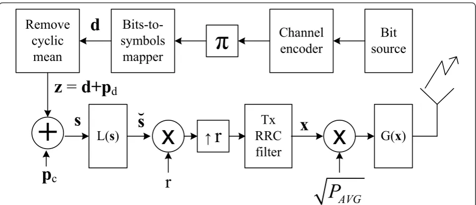
Our system design originates from the uplink assump-tion. Thus, the complexity of the transmitting end is kept as small as possible and most of the complexity is posi-tioned to the receiving end. The block level design of the transmitter is given in Figure 1. The transmitter contains a bit source, channel encoder, interleaver (represented by
πfunction), symbol mapper, pilot insertion, symbol level amplitude limiter,L(·), the transmitter pulse shape filter and nonlinear amplifier,G(·).
Let us assume that our symbol mapper produces a vector of data symbols d from some finite alphabet AN,
where N is the frame (vector) length. We will use a pilot sequence, p, which has length Np. The pilot sequence is an optimal channel independent (OCI) sequence that was defined in [2], and rewritten here as
p(k) =σpej
π
Np[k(k+v)], (1)
wherek = 0,...,Np- 1,v= 1 if Npis odd andv= 2 if
Np is even number. In addition, we assume that our frame length is an integer multiple ofNp, givenas N=
NcNp, where Nc is the number of cyclic copies per frame. With the DDST, we first remove the cyclic mean of the data vector. As shown in [4], this can be expressed as
z= (I−JTx)d, (2)
limiter from which the limited signal s is then obtained. This sequence is then oversampled with rater, given as
sr=rs⊗r, and inserted to the transmit pulse shape filter
to obtain transmitted sequencex. We define the power of the data sequence to be σ2
d = 1−γ and the power of the
known pilot sequence to be σpc2 =γ, wheregis the pilot
power allocation factor.
The peak amplitude limiter is presented by a functionL
(·), which takes as the maximum allowed amplitude value,
amax, the maximum amplitude value of the used
constella-tion A, defined as {amax= max((d)),d∈A,σd2= 1}.
We use this value because we wanted to achieve similar type of PAPR behavior as with TDMT and that the limiter affects mainly pilot sequences added on top of the user data. The limited symbol sequence can be defined as
s(k) =L(s(k)) =
s(k), ifs(k)≤amax,
amax·exp(j s(k)), ifs(k)>amax.(3)
Now we have an amplitude limited symbol sequence whose PP is limited to the same value as the original data symbol sequenced. The average power decrease, and the remaining PAPR increase, depends on the constellation. This kind of amplitude limiter, which keeps the argument difference between input and output as a constant, realizes so-called amplitude-modulation to amplitude-modulation (AM-AM) conversion [10], meaning that |L(s(k))| depends only on |s(k)|.
We have chosen to study the hard limiting of the trans-mitted symbols, but of course other limiters with differ-ent input-output mappings require more studies. Furthermore, we have chosen to study symbol level
limiting instead of limiting the output of the Tx pulse shape filter, which is a more common approach for con-trolling the PAPR in SC transmission. From the literature concerning studies on PAPR with OFDM modulation, one can find several possible topics of study in order to reduce PAPR in DDST with a modified data-dependent pilot sequence, and these are left for future studies.
Let us define an error vector elimiter=s−s, which contains the information removed by the limiter from the sequences. It represents an additive error sequence generated by the limiter. This model is used when we present the receiver feedback structure in Section 7.
The signal after the symbol level limiter, s, is then fed to the transmit pulse shape filter after over-sampling. We have used traditional root-raised-cosine (RRC) filter-ing with rolloff factor r= 0.1 and filter order NRRC=
64. We have chosen two different scenarios for simula-tions. For the PAPR and spectral leakage simulations we have used four times oversampling,r = 4, and for the performance evaluations we have used two times over-sampling, r = 2. We have chosen this setup for better understanding of the spectral spreading and because the used filter bank (FB) based equalizer is designed to work with two times oversampled sequences.
The nonlinear power amplifier model is a widely-used basic model, based on solid-state power amplifier (SSPA) model by Rapp [11]. The AM-to-AM conversion function for an input amplitudeAis given as
G(A) =v A 1 +vAA
0
2p−2p, (4)
%LW
VRXUFH
&KDQQHO
HQFRGHU
ʌ
%LWVWR
V\PEROV
PDSSHU
7[
55&
ILOWHU
5HPRYH
F\FOLF
PHDQ
G
V
S
F
V
Ù
]
GS
G
/
V
[
Ĺ
U
[
*
[
U
[
AVG
P
where v is the small signal amplification, A0 is the
saturation amplitude of the amplifier andpdefines the smoothness of the transition from linear region to the lim-iter region. The actual values chosen for the simulations are discussed in more detail in Section 7.
Based on Bussgang’s theorem [12], we model the output of the power amplifier as G(x) =αPAVGx+nG, wherea
is a scaling factor for the input signal,PAVGis the average
power of the transmitted frame, andnGis uncorrelated Gaussian noise vector caused by the nonlinear power amplifierG(·).PAvgis used to scale the average power of
the transmitted frame in order to stay inside the spectral mask to be defined in Section 5. The Bussgang’s theorem is based on Gaussian variables, but it’s results are widely used, e.g., in PAPR modeling for orthogonal frequency domain multiplexing (OFDM) systems. Also in our case, the signals are not purely Gaussian, but after the pulse shape filter they are Gaussian like and we can apply Buss-gang’s theorem to model the non-linear limiting caused by the power amplifier model.
We have assumed a discontinuous block wise transmis-sion where the channel is assumed to be time invariant during the transmission time of one frame. The used channel model is a modified ITU-R Vehicular A channel [13].
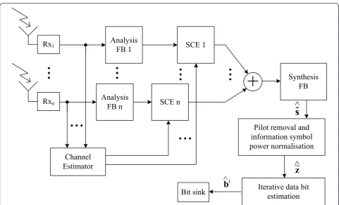
In Figure 2, we have presented a block diagram of our multiantenna receiver. We have extended the model pro-vided in [4] to our SC model with FB-based frequency-domain equalizer structure, presented in [14]. The analysis FB converts the time domain signal to the frequency domain (similar to the well known DFT operation) and the synthesis FB converts the frequency domain presenta-tion back to time domain (similar to the IDFT operapresenta-tion). The channel estimates are obtained in time domain after which the sub-channel wise equalization (SCE) is per-formed in the frequency domain with 3-tap complex FIR filter for each sub-channel. The equalizers for each diver-sity branch are designed based on the maximum ratio combining (MRC) criteria, presented in [15]. The channel estimates could also be obtained in the frequency domain and after suitable interpolation with DDST they could be directly used for defining the SCE equalizer tap values for each sub-channel. The FB-based receiver structure is used because it does not require a cyclic prefix (improved throughput), provides close to ideal linear equalizer per-formance, has good spectral containment properties (adja-cent channel suppression is clearly better than with DFT based solutions) and is equally applicable also to SC-FDMA (DFT-S-OSC-FDMA) as used in 3GPP-LTE uplink.
We assume perfect synchronization in frequency and time domain and ideal down conversion of the received signal in theRxblock. Several studies on DDST suitability for time and frequency synchronization have been
performed, e.g., [16,17], where it has been shown that DDST is also a viable solution for low SNR synchroniza-tion. We can present the channel between transmitter and receiver as anrtimes oversampled discrete-time equivalent channel,heq(n) = |hRRC(t)○hchannel(t)○hRRC(t)|t=nT/r= |
hRRC○hchannel+RRC|t=nT/r. Thenth received sampleyi(n) from theith antenna can be given as
yi(n) =α
where M is the channel length in samples, n is the time index forrtimes oversampled symbol sequence,nG (n) is a noise term caused by the nonlinear amplifier, and sr(n) is a possibly limited, oversampled transmitted
symbol, which is zero if n< 0 orn>rN - 1. The noise term wi(n) is complex additive white Gaussian noise (AWGN). Because of the r times oversampling, in our cases(k) =d(k) =pd(k) =pc(k) = 0 whenkmodulus r≠ 0. The channel estimation procedures are simply repeated for each diversity branch. For this reason and for the sake of clarity, we drop out the antenna indexi.
We can now rewrite the received discrete-time signal in the matrix notation as
y=αPAVG
Srheq+NGhchannel+RRC+WhRRC, (6)
where the matrix Sr=Dr+Pd,r+Pc,r+Elimiter,r is built
from the oversampled user data symbols, data depen-dent pilot sequence, known cyclic pilot sequence and the additional error generated by the symbol level lim-iter (only with LDDST), respectively. Here NG and W are the matrix presentations of the amplifier induced and channel induced noise terms, respectively.
including the zeros before and after the transmitted frame. Note that the oversampled matricesDr, Pd,r,Pc,r, Elimiter,r are now of dimension (rN + rNp ×rNp) and that we have assumed thatM=rNp. This means that in the receiver we have to do the cyclic mean calculation over Nc + 1 copies. Thus, the cyclic mean of the received sequence is given as
ˆ
my=JRxy
=αPAVG[Pr+Mˆelimiter,r]heq
+MˆnGhchannel+RRC+MˆwhRRC,
(8)
where JRx= (1/Nc)11×Nc+1⊗IrNp. In our notation, for any vector b, the cyclic mean vector is defined as
ˆ
mb=JRxb= [mˆb(0)mˆb(1). . .mˆb(rNp−1)]T, and for
any matrixB, the cyclic mean matrix is defined as
ˆ
Mb=JRxB=
⎡ ⎢ ⎢ ⎢ ⎣
ˆ
mb(0) mˆb(rNp−1)· · · ˆmb(2)mˆb(1)
ˆ
mb(1) mˆb(0) · · · ˆmb(3)mˆb(2) ..
. ... . .. ... ...
ˆ
mb(rNp−1)mˆb(rNp−2)· · · ˆmb(1)mˆb(0)
⎤ ⎥ ⎥ ⎥
⎦. (9)
For example, if you setb =elimiter,r, then Mˆelimiter,r is a
cyclic matrix having mˆelimiter,r as the first column. The
pilot matrix Pr is a cyclic matrix, having the r times
oversampled OCI pilot sequence pr=rp⊗ras its first column.
From the receiver frontend, the oversampled signal is provided for the channel estimator and for the analysis FB. After obtaining a channel estimate, SCE is per-formed in the frequency domain. More details on the equalizer structure can be found from [14,18], and refer-ences therein. After the SCE, different antenna branches are added together sub-channel wise according to the MRC principle. The composite sub-channels are then recombined in the synthesis FB, which also efficiently realizes the sampling rate reduction by 2.
After the synthesis FB, we have the Pilot removal and information symbol power normalization block. Inside this block, the received sequence power is normalized to
σ2 ˆ˜
s = 1 +σ
2
whRRC
2
, which corresponds to the total received power. We have assumed that we exactly know the noise variance in the receiver. Next, we scale the power based on the pilot power allocation and remove the cyclic mean of the received sequence. If we use LDDST, we normalize the sequence based on our esti-mate on the average transmit power σ2
s, to be defined
in (18), to obtain an estimate for the distorted data sequence,
5[
5[
Q$QDO\VLV
)%
$QDO\VLV
)%Q
&KDQQHO
(VWLPDWRU
6&(Q
6&(
6\QWKHVLV
)%
3LORWUHPRYDODQG
LQIRUPDWLRQV\PERO
SRZHUQRUPDOLVDWLRQ
%LWVLQN
E
,WHUDWLYHGDWDELW
HVWLPDWLRQ
LA
]
A
a
Ù
V
A
ˆ˜
Here zˆ˜ is an estimate for zwith cyclic mean set to zero and including the limiter error. Note that the cyclic mean of the limiter error is also zero.
Next, we have the Iterative data bit estimation block, where we iteratively obtain the data bit estimates. The procedures performed inside this block are described in detail in Section 6. Finally, the bit estimates are col-lected for bit error rate (BER) and block error rate (BLER) evaluations. The concept of (data) block in our system will be described in more detail in Section 7.
3 Symbol level limiter error modeling
Even though the earlier discussion assumed that the error caused by the symbol level limiter is purely addi-tive, we will adopt an another model for the channel estimator modifications. In this Section, we will assume that symbol level amplitude limiter will only affect the data dependent pilot sequence, pd, and cyclic pilot sequence,pc. We model the effects by a common scal-ing factor and added noise. We refer to this model as the double-scaling model. We start by rewriting the lim-ited symbol sequence as
s=L(s) =d+β(pd+pc) +nL. (11)
Here the additive noise component caused by the lim-iter,nL, is assumed to be uncorrelated withpd andpc, and it is assumed to have complex Gaussian distribu-tion. This model is a rough approximation of the phe-nomena that take place in the symbol level limiter, but based on our experience it provides sufficient accuracy for the channel estimator. The main difficulty in the modeling is to incorporate the effect of the limiter on the random data-dependent pilot sequence. We have tried several models, but they all have similar or worse accuracy than the Gaussian model we are going to pre-sent here, so we chose it because of its simplicity.
We can rewrite the purely additive limiter error given in the previous Section as elimiter=s−s= (β−1)(pd+pc) +nL. The cyclic mean of the received sequence can now be rewritten as
Because we have assumed that the limiter would affect only the pilot sequences, we have to define new methods for approximating these scaling parameters. We approxi-matebby generating a symbol vector consisting of all pos-sible data symbol and pilot symbol combinations, defined as scomb,1=(1−γ)dl+√γpl= 1Np×1⊗d+p⊗12Q×1, whered is a vector containing all possible symbols,pis the OCI pilot sequence andQis the number of bits per symbol. Next, we run this test sequence through the lim-iter and approximate the scaling factor as
β= p
H
l L(scomb,1)
pHl pl
, (13)
where we basically calculate a correlation based weighting factor for the extended pilot sequence,pl. We use this same weighting factor for data dependent pilot sequence because it undergoes similar effects in the symbol level amplitude limiter.
Now the difficult question is, how can we approximate
σ2
elimiter =E[
s−s2]. First we have to somehow model the distribution of the cyclic mean of the transmitted sequence. The probability of a certain combination of
Ncsymbols follows the multinomial distribution p(x1,x2,. . .,xk;n,p1,p2,. . .,pk)
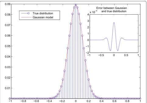
wherexiis the number of observations of a certain con-stellation point on a real or imaginary axis,piis the prob-ability of that constellation point and in our casen=Ncis the number of realizations in total per cyclic mean value. Herekis the number of constellation points per real or imaginary axis and takes the value of 2, 4 or 6 for QPSK, 16-QAM and 64-QAM, respectively. In this case, because all symbols are equally probable,pi= 1/kfor alli. To get the true probability of a certain cyclic mean value, one has to add together all the probabilities of different combina-tions leading to that specific cyclic mean value. With high number of cyclic copies, the distribution of the cyclic mean value tends toward the Gaussian distribution, as expected based on the central limit theorem. For this rea-son, we have chosen to model the data dependent pilot sequencepdwith a continuous complex Gaussian distribu-tionnpd∈N(0,σp2d), whereσ
is actually binomial), its Gaussian approximation and the error between these two models. The Gaussian approxi-mation is a good compromise for modeling purposes.
In order to approximate σe2limiter, let us first define
another symbol vector consisting of all possible data symbol and pilot symbol combinations, defined as
scomb,2=(1−1/Nc)(1−γ)dl+√γpl, where the
power scaling factor 1−1/Nc is used to ensure that
the total probability over the grid model, after adding Gaussian noise modeling the cyclic mean, equals to unity. Next, we add together probability grids, in which the different grids are based on the Gaussian distribution ofnpdcentered on a certain point of vec-tor scomb,2. The overall distribution can be given as
P(probability of symbolsscombat pointx,y)
=P(scomb,x,y) = step 2 2QNp
2QN p
k=1 1/
πσ2 pd
exp{1/σ2
pd[(Re (scomb,2(k))−x)
2+ (Im (scomb,2(k))−y)2]}, (15)
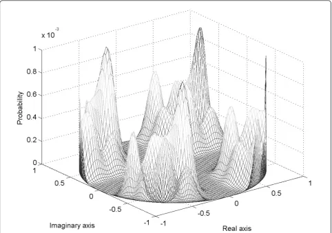
wherexandypresent the real and imaginary axes, respec-tively, in a grid with values from -2 to 2. The step size used for real and imaginary axis for calculating the probabilities of cyclic mean values from the Gaussian distribution is determined by the constellation, power normalization, pilot power allocation factor and the number of cycles used in the cyclic mean calculation. For example, if we are using 16-QAM constellation withg= 0.05 and have Nc= 80 cycles, the step size used isstep = 2√1−0.05/(80√10), where √10 is the power normalization factor to set 16-QAM constellation average power to unity. This step now corresponds to the smallest change in the cyclic mean over possible symbols in real or imaginary axis and directly pro-vides us a model for the discrete distribution of the cyclic mean with the defined parameters.
In Figure 4, we show as an example the generated grid model for QPSK constellation with pilot power alloca-tion factorg= 0.1 and number of cyclic meansNc= 80 after the limiter function. With QPSK the constellation power normalization factor is one, thus the step size is step = 2√0.9/80.
−1 −0.8 −0.6 −0.4 −0.2 0 0.2 0.4 0.6 0.8 1
0 0.01 0.02 0.03 0.04 0.05 0.06 0.07 0.08 0.09
−1 −0.5 0 0.5 1
−2
−1 0 1 2 3 4x 10
−4
Error between Gaussian and true distribution True distribution
Gaussian model
If we define g(x,y) =x2+y2 as a vectorized function
of the distances of grid points (x, y) from the origo, we can approximate σe2limiter, given as
σ2
elimiter =
x,y
g(x,y)−L(g(x,y))2P(scomb,x,y). (16)
We will use the σe2limitervalue in the ML-LMMSE
chan-nel estimator to incorporate a priori knowledge of the symbol limiter based error term.
If we now assume thatpc,pd, andnlimiterare
uncorre-lated, we can obtain the power of the limiter error with double-scaling model to be
σ2
nL =σ
2
elimiter−(β−1) 2(σ2
pd−σ
2
p)
=σe2limiter−(β−1)2(σd2/Nc−σp2).
(17)
By using the same grid model, we can obtain our esti-mate of the average power of the limited symbol sequence σ2
s
=E[s 2
], as
σ2
s
=
x,y
L(g(x,y))2P(scomb,x,y). (18)
Here, the average power of the amplitude limited sig-nal and the limiter error power could also be estimated by Bussgang’s method [12]. However, based on our simulations, the developed model gives similar estimates and is simpler because it does not require averaging simulations for the framewise correlation calculations. Thus, it provides an alternative approach to define these parameters.
4 Channel estimation with LDDST
In this Section, we will provide the used channel estima-tor for LDDST. When defining the LMMSE channel estimator, we want to minimize the expected value of the squared error, E{|ĥ - h|2}. If we now make the assumptions that the noise and the total interference experienced by the pilot sequence is AWGN, channel taps are i.i.d. and have zero mean, i.e., E{h} = 0, the LMMSE estimator can be simplified to [19]
Figure 4Example of the grid presentation for the probability distribution after the limiter function with QPSK modulation, cyclic OCI
ˆ models the total interference power based on the Gaus-sian channel noise, nonlinear power amplifier caused interference and the limiter error. The channel covar-iance matrix, Chˆ
apriori, contains the apriori information of
the channel tap values. The apriori information of the channel taps is obtained through a least squares (LS) channel estimator. From (12), the LS channel estimator can be defined as
ˆ
We have assumed independent tap coefficients, which allows us to model the apriori channel correlation matrix
Chˆ
apriorias a diagonal matrix. Because of the receiver pulse
shape filtering, this assumption is not exactly true, but it is used to provide us simpler diagonalized LMMSE esti-mator model, which reduces the channel estimation com-plexity. We shall refer to this LMMSE estimator, that uses LS based channel estimates as a priori information, as LS-LMMSE channel estimator. The performance of the receiver could be improved with more advanced methods taking the correlation into account, like the uni-versal basis based decomposition of the receiver pulse shape filter correlation, as was discussed in [20]. In a sense, the idea of using only the most significant compo-nents of the decomposition is similar to our idea of trun-cating the time window of the channel estimator to take into account only the most significant channel taps. Both methods gain in noise power reduction in the channel estimation but lose in the asymptotic accuracy.
In the channel estimator, we approximate the diagonal correlation matrix C by the instantaneous tap power obtained from the LS channel estimator, i.e.,
ChˆLS= diag By assuming the cyclic OCI training sequence, the LS-LMMSE estimator can be reduced to
ˆ
The variable σ2
est corresponds to the total interference
power on top of each received pilot symbol and is esti-mated as this value is unknown to the receiver. Similar channel estimator structure with traditional SI pilots and itera-tive interference canceling feedback was studied in [21].
5 PAPR analysis and spectral leakage comparison
One drawback with DDST in SC transmission is the increased PP and PAPR in the transmitted signal and spectral leakage caused by the non-linear amplifier due to the increased PAPR. These problems are well known but have received relatively little attention in the recent literature.
In a SC transmission, the PAPR of the transmitted sequence is defined after the Tx pulse-shape filter. The PP we see in the filter output depends on the maximum amplitude of the input symbols and on a portion of the absolute values of the filter coefficients, depending on the oversampling. Because we have fixed the Tx pulse-shape filter, only the maximum amplitudes of the input symbols effect the observed PAPR.
There are two main reasons for increased symbol level amplitude in DDST. First of all, we increase the ampli-tude range related to a certain constellation by adding a power scaled pilot sequence on top of a power scaled symbol sequence. The second main reason for increased amplitude is the possibility of a cyclic mean (data dependent pilot) component with relatively high ampli-tude. When this component is added on top of data and known pilot symbols, and if the angles of these complex variables happen to align, then the total symbol ampli-tude is significantly increased.
In this Section, we will first discuss the worst case PP and PAPR effects in more detail and after that we will describe the reference spectral power mask and related simulations and results.
5.1 PAPR analysis and simulated results
iis chosen based on criteria
transmit pulse shape filter of degree 64 andr = 4, the starting index which maximizes the sum-power isk= 2. Because the RRC filter acts also as a oversampling filter, the taps of the filter are multiplied by the oversampling factorr in order to keep the average transmitted power equal to unity.
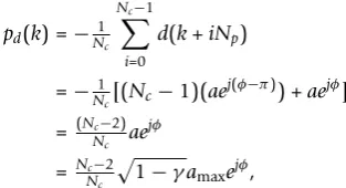
First, we define the worst case symbol level PP. Assume now thatd(k) =aejjis some corner symbol with ampli-tude aand all the other symbols present in the cyclic mean calculation,d(k+iNp) =aej(j-π)withi= 1,2,...,Nc -1, are opposite corner symbols with amplitudea. Then the data dependent pilot added on top ofd(k) is equal to
which corresponds to the worst case peak amplitude with the data dependent pilot sequence and its value depends on the used constellation and the pilot power allocation factorg. The worst case symbol level PP is defined for an aligned pilot√ pc(k) which has amplitude
γ. By aligned, we mean that the arguments of data and the pilot are equal,∠d(k) =∠pc(k) =j. Now we can write the worst case symbol level PP as
WPPs =d(k) +pd(k) +pc(k)2
=1 +Nc−2
Nc 1−γamax+
√γ2
. (26)
By using (26), we can define then the worst case PP after the transmit pulse shape filtering to be
WPPTx,DDST=
For TDMT, the worst case PP after the transmit pulse shape filtering is
If we use the presented hard symbol level limiter in the transmitter, then the worst case symbol level PP can be given as
WPPs,limited=L(d(k) +pd(k) +pc(k))
2
=a2max, (29) which is the same as with TDMT. Then the worst case PP after the RRC filtering is
WPPTx,DDST,limited=a2max
i∈i
hRRC(i) 2
. (30)
which is equal to TDMT case.
With the PPs defined, we can define the PAPRs for different cases. While reading the results for PAPR from Table 1, one should note the difference in the average powers used to define these PAPR results. The average power of a TDMT signal is given asE[|sTDM|2] = 1. For
DDST based system, the average power of the signal is E[|s|2] = (1−1/N
c)σd2+σp2. The weighting factor (1
-1/Nc) is caused by the removal of the cyclic mean from the data sequence. Now the worst case PAPR for DDST without limiter before and after the transmitter pulse shape filter can be given as
WPAPRs= EWPP[|s|2s]
The average power for LDDST is given as E[s
2
] =σ2
s
and is defined based on the Gaussian grid model in (18) in Section 3. The PAPRs for the limited case can be written as
WPAPRs,limited=
WPPs,limited
WPAPRTx,DDST,limited =
Finally, the PAPR for the TDMT case equals WPAPRTx,TDMT=
WPPTx,TDM
E[|sTDM|2]
=a2max
i∈i
hRRC(i) 2
.
(35)
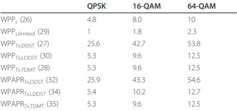
In Table 1, we have calculated different symbol level and transmitted signal related worst case PPs and PAPRs for different constellations with pilot power allocation factorg= 0.1. As we can see, the hard limiter significantly decreases the worst case PPs and PAPRs and the limited worst case PAPRs are close to the TDMT cases, as was desired.
If we assume that with DDST we want to set the PP at the transmit pulse shape filter output to be at a similar level as with TDMT, based on Table 1, a significant back-off is required. With symbol level amplitude limiter we can remove this backoff requirement. As a downside, the amplitude limiter causes additional interference in the transmitted symbols, which might be significant espe-cially with higher order modulations.
In Table 2, the different simulated PPs and PAPRs are given for each constellation. The simulated values were obtained by finding the maximum PAPR over 100,000 random frame realizations. These results provide more insight on the average PAPR performance of the given system with different training methods, and show that the defined analytic worst case PPs and PAPRs are reli-able upper bounds.
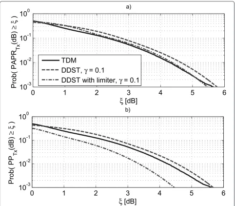
As expected, the PP and PAPR results with DDST are not as bad as the worst case studies suggested. The main benefit of using symbol level limiter seems to be with QPSK and 16-QAM constellations, where significant reduction in PAPR can be achieved. 64-QAM has quite similar performance with and without symbol level lim-iter. In Figure 5, an example of the complementary cumulative distribution functions (CCDF) for PP and PAPR distributions with QPSK constellation are shown.
Here we can see that the PAPR distributions are similar but the PP distributions are quite different.
5.2 Spectral leakage with SSPA amplifier model
In this section we will study the spectral re-growth with different training methods and with QPSK, 16-QAM, and 64-QAM constellations. The power amplifier model was given in Section 2. We have chosen to use valuesv= 1 andp= 3 for the simulations. Because we have assumed that the power amplifier is matched to work with TDMT transmission, we have set the 1 dB compression point of the power amplifier based on the 64-QAM constellation PP distribution. The chosen amplitude limit is related to the PP which gives us 1% probability in the CCDF. Thus, from the results obtained in the previous section, we can look for the PP with 64-QAM thatP(PP64-QAM≤P1dB) =
0.01. Based on our simulations, this value is equal toP1dB
= 4.8 dB. Now, we use this power value to solve the power amplifier saturation amplitude. The amplitude corresponding to the 1 dB compression point is A= 104.8/20and the saturation amplitude can be solved to be
A0=vA
10p/10−1 −10
2p
, (36)
which gives usA0 ≈1.739.
The used spectral mask is based on 3GPP technical spe-cification for E-UTRA user equipment [22]. The used required attenuation levels are based on 23 dBm transmis-sion power in the used 20 MHz bandwidth and Table 6.6.2.2.2-1 in page 44 of [22]. We chose the values of this Table because it provides the most strict attenuation mask. The obtained attenuation levels are given in Table 3 with respect to the distance from the channel band edge. This distance is defined as an out-of-band frequency dis-tance,ΔfOOB. The required attenuation levels are defined
for a measurement bandwidth of 1 MHz.
For the simulations, we have assumed to use 20 MHz channel bandwidth, 18 MHz symbol frequency and a roll-off factor 0.1 in the RRC filter. We wanted to keep
Table 1 WPP and WPAPR for the used constellations with
parameter valuesNc= 75,Np= 60, andg= 0.1
QPSK 16-QAM 64-QAM
WPPs(26) 4.8 8.0 10
WPPs,limited(29) 1 1.8 2.3
WPPTx,DDST(27) 25.6 42.7 53.8
WPPTx,LDDST(30) 5.3 9.6 12.5
WPPTx,TDMT(28) 5.3 9.6 12.5
WPAPRTx,DDST(32) 25.9 43.3 54.6
WPAPRTx,LDDST(34) 5.4 10.2 12.7
WPAPRTx,TDMT(35) 5.3 9.6 12.5
All values are given in linear scale
Table 2 Simulated PPs and PAPRs for the used
constellations with parameter valuesNc= 75,Np= 60,
andg= 0.1
QPSK 16-QAM 64-QAM
PPs 2.8 3.9 4.6
PPs,limited 1 1.8 2.3
PPTx,DDST 6.6 8.7 9.3
PPTx,LDDST 4.7 7.6 8.9
PPTx,TDMT 5.3 7.7 9.1
PAPRTx,DDST 6.8 9.0 9.5
PAPRTx,LDDST 5.9 8.2 9.2
PAPRTx,TDMT 5.3 7.8 9.2
the roll-off factor small because we are aiming toward very high spectral efficiency. For different training meth-ods and constellations, we ran the simulations looking for smallest IBO with 0.5 dB step in the average trans-mitted power,PAVG. We have defined the input backoff
(IBO) as IBO = 10log10(A2
0/PAVG). Based on the results,
we chose the smallest IBO for each training method and constellation which leads to spectral leakage that stays below the given spectral mask. The obtained IBO and output backoff (OBO) results are provided in the Table 4. The OBO is defined as the maximum output power to the average output power ratio, given as OBO = 10log10(A20/E[G(x)2]).
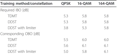
As expected, based on the PP and PAPR analysis, we can reach significantly lower OBO when using limited
DDST with QPSK constellation. With 16-QAM constel-lation we can decrease the OBO somewhat with symbol level limiter. With 64-QAM, meaningful gains were not achieved with symbol level amplitude limiter. These IBO values are used in Section 7 when we compare the throughput performance of different training methods.
Next, we will return to the actual implementation of the iterative receiver used with limited DDST before we study the throughput performance with different train-ing methods.
6 Iterative receiver algorithms
The receiver operations before the iterative data bit esti-mation were already described in Section 2. In this sec-tion we discuss in more detail the operasec-tions performed
0
1
2
3
4
5
6
10
-310
-210
-110
0ξ
[dB]
Pr
ob(
PAPR
Tx
(d
B
)
≥ξ
)
a)
TDM
DDST,
γ
= 0.1
DDST with limiter,
γ
= 0.1
0
1
2
3
4
5
6
10
-310
-210
-110
0ξ
[dB]
Pr
ob(
PP
Tx
(d
B
)
≥ξ
)
b)
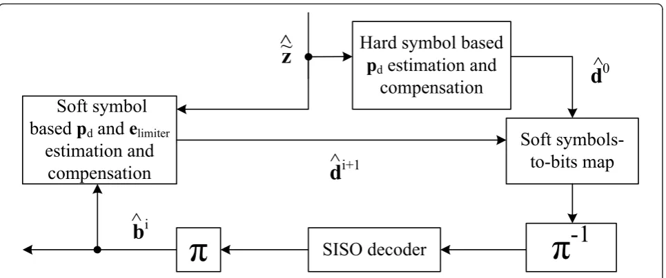
inside the iterative data bit estimation block, shown in more detail in Figure 6.
We have used notation zˆ˜ to represent our estimates of the data symbol sequence, including the limiter error, with cyclic mean set to zero, obtained from the pilot removal and information symbol power normalization block, as shown in Figure 2. We use zˆ˜ as a initial data symbol estimates to generate hard symbol based cyclic mean estimate in the hard symbol basedpd estimation and compensation block. Inside this block, we generate hard symbol estimates based on zˆ˜, calculate their cyclic mean and add it to zˆ˜, to obtain initial symbol estimates
ˆ
d0. Here superscript 0 points out that these symbol
esti-mates are obtained before coded feedback. This idea was presented in [4], and we use it before the first soft sym-bols to bits mapping.
We start the iterative reception process by using dˆ0to generate soft coded bit estimates bˆ˜ in thesoft symbols-to-bitsblock. These are then provided to the input soft-output (SISO) decoder from which we obtain our first soft decoded bit estimates to be provided for thepdandelimiter
estimation and compensation block and for bit error eva-luation. This block is presented in more detail in Figure 7, where superscriptirefers to the iteration number. These procedures, before we obtain the first feedback data sym-bol estimates, dˆ1, are considered to happen in the zeroth feedback iteration (i= 0). In our notation, after first pass through channel decoder, symbol estimation and compen-sation processes, we obtain our first feedback data symbol estimatesdˆ1, to be used for soft bit estimation.
The operations inside the pdand elimiter estimation
and compensation block, shown in Figure 7, are per-formed as follows. First we generate soft symbol esti-mates based on the latest soft bit estiesti-mates bˆi, which are equal to the log-likelihood presentation of the a pos-teriori probabilities obtained from the soft decoder. The soft symbols are given by equation
ˆ
where |A| gives the number of symbols in alphabetA,
νis a symbol index, bˆi
ν are the soft bit estimates related
to the νth symbol, and p
is the probability of a symbol da, given the latest soft bit estimates bˆiν. The probability of a symboldais defined as
pda| ˆb
where Q is the number of bits per symbol,
¯
bda(q)∈[−1, +1] is the qth bit of the hypothesis da, and bˆi
ν(q) is the log-likelihood presentation of the a
posteriori probability related to the qth bit of the νth symbol in theith iteration, given as
ˆ
We have also normalized the variance of the soft sym-bol vector, dˆi, to be equal to unity. This improves the
feedback performance when the soft bit estimates have very low reliability. In our simulations, using soft symbol feedback for the limiter error estimation provided better results than using hard symbol feedback.
Then, we calculate the symbol wise cyclic mean and remove it from the symbol sequence to obtain zˆi. Now
− ˆpid is an improved estimate of the cyclic mean, assum-ing that the SISO decoder has been able to reduce the number of bit errors in the detected bit sequence. Next, we add the known pilot sequence on top of the sequence zˆi to get ˆ
si and provide this sequence to the
amplitude limiter. Then we calculate the limiter error estimate based on the input and the output of the lim-iter function and an improved estimate of the average power, σ2
ˆ
s
i. At this point, when i > 0, we obtain our first estimate of the limiter error. Based on our results, it is better to estimate the limiter error after the channel
Table 3 Attenuation at distanceΔfOOBfrom the channel
band edge
ΔfOOB[MHz] Attenuation requirement [dB]
±0-1 -15.76
±1-5.5 -22.99
±5.5-25 -34.99
Table 4 Simulation based IBO and OBO results for different training methods and constellations
Training method/constellation QPSK 16-QAM 164-QAM
Required IBO [dB]
TDMT 5.3 5.8 5.8
DDST 5.3 5.8 5.8
DDST with limiter 3.8 5.3 5.8
Corresponding OBO [dB]
TDMT 5.5 6.0 6.0
DDST 5.6 6.1 6.1
DDST with limiter 5.0 5.8 6.1
decoder and not based on the uncoded hard symbol estimates dˆ0. With low code rates (lowEb/N0 region)
the uncoded limiter error estimation leads to worse per-formance in all iterations. Then again, with high code rates (highEb/N0 region) uncoded limiter error
estima-tion improves the BLER performance at the 0th itera-tion, but the iterative gain decreases, leading to worse performance at the fifth iteration.
Based on this improved average amplitude estimate, we can obtain improved symbol estimates by rescaling the average power of the received sequence, remember-ing that we have already scaled the incomremember-ing sequence by σ
s in (10). Finally, we can generate new symbol
estimates by adding to the received symbol estimates zˆ˜ the latest cyclic mean and limiter error estimates, given as
ˆ
di+1=
σ
ˆ
s
i
σ s
ˆ˜
z− ˆ˜eilimiter− ˆp
i d
=
σ
ˆ
s
i
σs ˆ˜
z−(I−JTx)eˆilimiter+JTxdˆ i
.
(40)
We remove the cyclic mean of the estimated limiter error eˆilimiter, because we have completely removed the cyclic mean from zˆ˜, including the limiter error.
6RIWV\PEROV
WRELWVPDS
6,62GHFRGHU
ʌ
6RIWV\PERO
EDVHG
S
GDQG
H
OLPLWHUHVWLPDWLRQDQG
FRPSHQVDWLRQ
ʌ
E
LA
G
LA
]
A
a
+DUGV\PEROEDVHG
S
GHVWLPDWLRQDQG
FRPSHQVDWLRQ
G
A
Figure 6A block diagram presenting the operations performed inside the Iterative data bit estimation.
6RIWV\PEROV
WRELWVPDS
6,62GHFRGHU
ʌ
6RIWV\PERO
EDVHG
S
GDQG
H
OLPLWHUHVWLPDWLRQDQG
FRPSHQVDWLRQ
ʌ
E
LA
G
LA
]
A
a
+DUGV\PEROEDVHG
S
GHVWLPDWLRQDQG
FRPSHQVDWLRQ
G
A
Based on our results, it is better not to use the extrin-sic information obtained from the channel decoder as a priori information in the soft symbols-to-bits mapping, if this information is already used to improve the cyclic mean estimate. This is probably because we are using the same information twice inside the same loop, thus losing the independence of the a priori information. We can use it as a priori information if we do not improve the cyclic mean, but based on our studies this does not provide as good iterative gain in the receiver. This could be because of the error averaging nature of the cyclic mean computation.
Here we remind the reader, that even without symbol level amplitude limiter, we have to use iterative detec-tion algorithm for the cyclic mean estimadetec-tion. Of course, the limiter error estimation is not required. Therefore, in the simulation results presented in Section 7, the throughput results obtained with DDST also include five feedback iterations.
For a reader interested in a pure SI training with itera-tive reception, a good starting point is, for example, [23]. In this article a computationally efficient, iterative fre-quency-domain equalization and channel estimation is presented. In this article, we have not considered of including the channel estimation process in the iterative loop because with DDST there is no interference from the data symbols to the known pilot symbols. Nonethe-less, when there is symbol level limiter involved, we could feedback the cyclic mean of the limiter error esti-mate in order to improve the channel estiesti-mates with LDDST. In addition, in SISO case or in spatially multi-plexed MIMO case, the feedback filtering used also in [23], is of great interest and provides interesting topics for future research.
7 Performance comparisons
In this section, we will first provide some results demon-strating the performance of our iterative receiver algo-rithm. In the end, spectral efficiency comparisons between TDMT and DDST based training are provided. This is, after all, the most important topic of this article. We will investigate whether the end user spectral effi-ciency is really improved with DDST and do we gain something by using a symbol level amplitude limiter.
The used channel model is a block-fading extended ITU-R Vehicular A channel with approximately 20 MHz bandwidth [13]. The maximum delay spread of the chan-nel is 78 samples. In [13], the chanchan-nel model was defined for sampling intervalts= 32.55 ns where as in our system the sampling interval ists= 27.78 ns. This modification has a minor effect on the spectral correlation properties of the channel. However, the main idea is only to do some initial comparisons in the possible throughput per-formance between DDST and TDMT training based
systems. Therefore, the used model provides a good starting point for the simulations.
The oversampling in the receiver allows us to effi-ciently realize the RRC filtering in frequency domain in combination with the channel equalization process. More details can be found in [14] and references therein. In this article we have considered single-input single-output (SISO), and 1 × 2 and 1 × 4 single-input multiple-output (SIMO) antenna configurations with MRC equalizer.
In our simulations, the channel estimator length isrNp = 120 while the true equivalent channel length, includ-ing the effects of transmitter and receiver RRC filters, is
Nchannel+ 1 + 2NRRC = 206 samples. This kind of short
channel estimator was studied in [21,24]. The reason behind using short channel estimator is to maximize the number of cycles, Nc, with the cost of minimizing the estimator length, Np. Because we are estimating the equivalent channel, we can ignore channel tap values close to zero, which are caused by the heavy tailing of the RRC filters. In the presented simulations we have used values Nc = 75 and Np = 60 with DDST and LDDST. This gives us a good compromise with the esti-mator accuracy and achievable number of cyclic copies. Especially with QPSK modulation, when we are working in a high noise environment, it is worth to consider sacrificing the channel estimation accuracy to achieve better noise power averaging through increased number of cyclic copies. With higher order constellations, in addition to the improved noise averaging, with increased number of copies we can also decrease the variance of the data dependent training sequence, pd, and this improves the accuracy of the first symbol estimates.
The channel codec uses turbo code [25] with generator matrixG= [11 51 3]. We have used the max-log-MAP algo-rithm presented in [26] without any correction factor for the max-operator. The extrinsic information exchanged between the component decoders is weighted by a factor 0.75 to reduce the error propagation, as proposed in [27]. Iterations in the turbo decoder are terminated based on the hard-data-aided algorithm presented in [28]. The used interleavers are bitwiseS-interleavers [29], where the distance parameter is defined as S=U/2whereU
is the length of the unit which is interleaved. In channel interleaving the unit is the whole transmitted frameU=
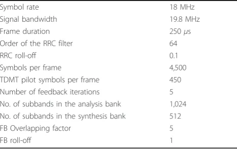
We have run the simulations for QPSK, 16-QAM, and 64-QAM constellations with code rates R = 0.5, R= 0.67 and R= 0.75. With TDMT pilots, the number of transmitted data symbols in each frame is decreased by the number of pilot symbols, which is set to be 450 in our simulations (10% of the frame duration). The TDMT pilots are the first 450 binary symbols from a Gold code of length 512 symbols [31] with unity power. The channel estimator length is equal to the equivalent channel length. With DDST, we decided to provide same portion of total power for the pilots, thusg = 0.1. This gives us a fair comparison between TDMT training and DDST based transmission, because the channel esti-mation MSE of basic least-squares channel estimator with DDST is the same as with TDMT, if equal amount of power is allocated for the pilots [4]. The optimization of the pilot powers with TDMT or DDST for channel estimation with transmitted average power and PP restrictions is an interesting and open problem, but is out of the scope of this article. Some additional simula-tion parameters related to the simulasimula-tion model are given in Table 5.
In all the simulated cases we have used the maximum of five feedback iterations for pˆd and êlimiterestimation.
Typically, for QPSK modulation two and for 16-QAM modulation three feedback iterations already provide relatively good performance. With 64-QAM modulation we need five feedback iterations to ensure convergence in all of the cases. Example of the typical BLER behavior over iterations with LDDST using amplitude limiter with different constellations, compared to TDMT, is shown in Figure 8. We have assumed that the receiver does not know the IBO used in the transmitter and this degrades the performance results in all of the simulated cases.
One rather intriguing problem while planning the spec-tral efficiency comparison was the choice of the reference power. The comparison of performance with DDST and TDMT based systems is not so trivial and one has to be
careful about what to compare and how these results should be interpreted.
In the simulations, we chose to do the performance comparisons with respect to the energy per transmitted data bit over one sided noise spectral density, Eb/N0.
We have chosen this parameter because what matters most in modern wireless communications is the used energy per data bit to transmit with certain spectral effi-ciency. We have defined the SNR based onEb/N0as
SNR = EbQRtrue N0r
, (41)
whereQis the number of bits per symbol,Rtrueis the
true coding rate (including the effect of possible termina-tion bits, block length modificatermina-tions with zero padding, etc.), and r = 2 is the oversampling rate used in the receiver.
Figures 9 and 10 present spectral efficiency results for DDST, LDDST and for TDMT training, using also a LS-LMMSE type equalizer, with QPSK modulation and with 16-QAM and 64-QAM modulations, respectively. From Figure 9 we can observe how the increased average trans-mit power allowed by the symbol level amplitude litrans-miter improves the spectral efficiency in the lowEb/N0range
with QPSK modulation. In Figure 10 we have shown the performance with higher order modulations. Here, the performance of LDDST compared to DDST is quite simi-lar. Clearly, both DDST based systems improves the spectral efficiency over the wholeEb/N0 range for each
antenna configuration. The maximum spectral efficiency difference for each constellation is equal to 10%, which corresponds to the pilot overhead of TDMT.
With the proposed symbol level amplitude limiter we can obtain improved spectral efficiency performance with QPSK modulation in all antenna configurations. With 16-QAM or 64-QAM modulations, LDDST and DDST have quite the same performance. Possibly, one could improve the LDDST performance with higher order modulations by tighter limiting bounds. In addition, by first performing tighter limiting and after that removing the cyclic mean, we could decrease the limiter error effect in the channel estimation and possibly improve the sys-tem performance. These topics are left for future studies.
8 Conclusion
In this article, we have discussed the effects of a DDST based training on the signal PP and PAPR distributions. We demonstrated that the PP and PAPR distributions of the DDST based training have longer tails and therefore there is a higher probability for big PAPR values. Espe-cially, with constant amplitude modulations like QPSK, the average PAPR is significantly increased. Furthermore, the effects of the increased PAPR on the spectral leakage
Table 5 Simulation parameters
Symbol rate 18 MHz
Signal bandwidth 19.8 MHz
Frame duration 250μs
Order of the RRC filter 64
RRC roll-off 0.1
Symbols per frame 4,500
TDMT pilot symbols per frame 450 Number of feedback iterations 5 No. of subbands in the analysis bank 1,024 No. of subbands in the synthesis bank 512
FB Overlapping factor 5
5HPRYH
F\FOLF
PHDQ
S
F6RIW
V\PERO
PDSSHU
5HFHLYHG
GDWD
V\PERO
HVWLPDWH
1HZGDWDV\PERO
HVWLPDWHVWREH
XVHGIRUVRIWELW
HVWLPDWLRQ
E
A
LG
A
LA
]
LA
V
LA
V
Ù
L
A
S
LGH
A
LOLPLWHU5HPRYH
F\FOLF
PHDQ
H
Aa
LOLPLWHU[
G
A
LA
]
A
Ù
]
A
]
a
ˆ
is
s
σ
σ
/DWHVWGDWDELW
HVWLPDWHVIURPWKH
6,62GHFRGHU
Figure 8BLER for QPSK, 16-QAM, and 64-QAM with two receiving antennas and with code rateR= 0.75 using LDDST or TDMT.
2
4
6
8
10
12
14
16
18
10
−310
−210
−110
0BLER
E
b
/N
00th iteration
1st iteration
2nd iteration
3rd iteration
4th iteration
5th iteration
TDMT
with SSPA amplifier model were studied. It was shown, that DDST does not require higher IBO compared to TDMT, but does provide slightly worse OBO perfor-mance. The proposed symbol level limiter can decrease further the IBO and OBO requirements with QPSK and 16-QAM constellations. The reduced OBO and IBO may significantly ease the design, implementation and cost of the required power amplifier. With QPSK modulation the symbol level limiter also clearly decreases the spectral re-growth and improves the spectral efficiency perfor-mance via higher average transmitted power.
Based on our results, with QPSK and 16-QAM, one should consider using LDDST to allow higher average transmitted power (lower OBO) and to achieve improved throughput compared to DDST. With higher order constellations symbol level amplitude limiter, as
presented in this article, doesn’t seem to provide signifi-cant benefit.
With DDST, with or without symbol level amplitude limiter, the complexity increase compared to traditional TDMT training can be approximated by the complexity of the SISO decoder used. In the soft feedback loop with DDST, with or without symbol level amplitude limiter, the SISO decoder is dominating the detection complexity. Thus, the average increase in the detection complexity compared to TDMT, is roughly the average number of feedback iterations times the number of blocks decoded in average in each feedback iteration times the average com-plexity of decoding one block in the SISO decoder. With TDMT no feedback iterations are required.
The performance comparisons between DDST and TDMT based system showed that DDST can provide
3
4
5
6
7
8
9
10
11
0
0.5
1
1.5
E
b/N
0[dB]
TDM
DDST
LDDST
0
1
2
3
4
5
6
0
0.5
1
1.5
E
b
/N
0[dB]
Spectral efficiency [bits/s/Hz]
−
0
3
−
2
−
1
0
1
2
0.5
1
1.5
E
b
/N
0[dB]
1 Rx Antenna
2 Rx Antennas
4 Rx Antennas
similar or better performance over the whole Eb/N0
range with all antenna configurations. The proposed symbol level amplitude limiter improves the throughput performance of the DDST in the low Eb/N0range with
all antenna configurations tested.
In addition to careful performance analysis and com-parisons, we have provided some new ideas for PAPR control with DDST, for modeling the effects of symbol level limiter in channel estimation, and for modeling the cyclic mean distribution based on multinomial distribu-tion or its Gaussian approximadistribu-tion.
Acknowledgements
The authors would like to thank Dr. Ali Shahed Hagh Ghadam for enlightening the mysteries of power amplifiers. This work was supported by the Tampere Graduate School in Information Science and Engineering (TISE), the Nokia Foundation and the Academy of Finland (under Project No. 129077,“Hybrid Analog-Digital Signal Processing for Communications Transceivers”).
Competing interests
The authors declare that they have no competing interests.
Received: 11 May 2011 Accepted: 16 February 2012 Published: 16 February 2012
References
1. P Hoeher, F Tufvesson, Channel estimation with superimposed pilot sequence, inProc IEEE Global Telecommunications Conference 1999
GLOBECOM‘99, vol. 4. (Janeireo, Brazil, 1999), pp. 2162–2166
2. AG Orozco-Lugo, MM Lara, DC McLernon, Channel estimation using implicit training. IEEE Trans Signal Process.52(1), 240–254 (2004). doi:10.1109/ TSP.2003.819993
3. SAK Jagannatham, BD Rao, Superimposed pilot vs. conventional pilots for channel estimation, inFortieth Asilomar Conference on Signals Systems and
Computers 2006 ACSSC‘06, (Pacific Grove, California USA, 2006), pp. 767–771
4. M Ghogho, DC McLernon, E Alameda-Hernandez, A Swami, Channel estimation and symbol detection for block transmission using data-dependent superimposed training. IEEE Signal Process Lett.12(3), 226–229 (2005) 5. DC McLernon, E Alameda-Hernandez, AG Orozco-Lugo, MM Lara,
Performance of data-dependent superimposed training without cyclic prefix. Electron Lett.42(10), 604–606 (2006). doi:10.1049/el:20060127 6. E Gayosso-Rios, MM Lara, AG Orozco-Lugo, DC McLernon, Symbol-blanking
superimposed training for orthogonal frequency division multiplexing systems, in7th International Symposium on Wireless Communications Systems
(ISWCS), York, UK, pp. (19–22 Sept 2006), 204–208
7. C-T Lam, DD Falconer, F Danilo-Lemoine, R Dinis, Channel estimation for SC-FDE systems using frequency domain multiplexed pilots, inIEEE 64th Vehicular
Technology Conf 2006 VTC-2006 Fall, (Montreal, Canada, 2006), pp. 1–5
8. T Levanen, J Talvitie, M Renfors, Performance evaluation of a DDST based SIMO SC system with PAPR reduction, in6th International Symposium on
Turbo Codes & Iterative Information Processing, ISTC 2010, (Brest, France,
2010), pp. 186–190
9. DC McLernon, E Alameda-Hernandez, A Orozco-Lugo, MM Lara, New results for channel estimation via superimposed training, inProc Second International Symposium on Communications Control and Signal Processing
ISCCSP 2006, (Marrakech, Morocco, 2006). (Article ID cr1001). ISBN:
2-908849-17-8
10. R Raich, H Qian, GT Zhou, Optimization of SNDR for amplitude-limited nonlinearities. IEEE Trans Com-mun.53(11), 1964–1972 (2005)
11. C Rapp, Effects of HPA-nonlinearity on a 4-DPSK/OFDM-signal for a digital sound broadcasting system, inSecond European Conference on Satellite
Communications, ECSC-2, (Liege, Belgium, 1991), pp. 179–184
12. JJ Bussgang, Crosscorrelation functions of amplitude-distorted gaussian signals, (Technical report (Massachusetts Institute of Technology. Research Laboratory of Electronics), 1952) Report no.:216,
13. TB Sorensen, PE Mogensen, F Frederiksen, Extension of the ITU channel models for wideband (OFDM) systems, inIEEE 62nd Vehicular Technology
Conference 2005 (VTC-2005-Fall), (Dallas, Texas, USA, 2005), pp. 392–396
14. Y Yang, T Ihalainen, M Rinne, M Renfors, Frequency-domain equalization in single-carrier transmission: filter bank approach. EURASIP J Adv Signal Process (2007).2007, (Article ID 10438)
15. MV Clark, Adaptive frequency-domain equalization and diversity combining for broadband wireless communications. IEEE J Sel Areas Commun.16(8), 1385–1395 (1998). doi:10.1109/49.730448
16. E Alameda-Hemndez, DC McLernon, AG Orozco-Lugo, MM Lara, M Ghogho, Improved synchronization for superimposed training based channel estimation, inIEEE/SP 13th Workshop on Statistical Signal Processing, (Bordeaux, France, 2005), pp. 1324–1329
17. SMA Moosvi, DC McLernon, AG Orozco-Lugo, MM Lara, M Ghogho, Carrier frequency offset estimation using data-dependent superimposed training. IEEE Commun Lett.12(3), 179–181 (2008)
18. Y Yang, T Ihalainen, M Renfors, Filter bank based frequency domain equalizer in single carrier modulation, inProc 14th IST Mobile & Wireless
Communications Summit, (Dresden, Germany, 2005)
19. M Pukkila, Iterative Receivers and Multichannel Equalisation for Time Division Multiple Access Systems, Ph.D. dissertation, (Helsinki University of Technology, Espoo, Finland, 2003) ISBN 951-22-6717-9
20. R Carrasco-Alvarez, R Parra-Michel, AG Orozco-Lugo, JK Tugnait, Enhanced channel estimation using superimposed training based on universal basis expansion. IEEE Trans Signal Process.57(3), 1217–1222 (2009)
21. T Levanen, M Renfors, Improved performance bounds for iterative IC LMMSE channel estimator with SI pilots, in21st Annual IEEE International
Symposium on Personal Indoor and Mobile Radio Communications, (Istanbul,
Turkey, 2010), pp. 9–14
22. 3GPP TS36.101 V10.1.0 (2010-12), 3rd Generation Partnership Project; Technical Specification Group Radio Access Network; Evolved Universal Terrestrial Radio Access (E-UTRA); User Equipment (UE) radio transmission and reception (Release 10) http://www.3gpp.org/ftp/Specs/archive/ 36_series/36.101/36101-a10.zip (2012)
23. R Dinis, C-T Lam, D Falconer, Joint frequency-domain equalization and channel estimation using superimposed pilots, inIEEE Wireless Communications
and Networking Conference (WCNC), (Las Vegas, NV, USA, 2008), pp. 447–452
24. T Levanen, J Talvitie, M Renfors, Improved performance analysis for super imposed pilot based short channel estimator, inIEEE International Workshop
on Signal Processing Advances for Wireless Communications SPAWC 2010,
(Marrakech, Morocco, 2010), pp. 1–6
25. C Berrou, A Glavieux, P Thitimajshima, Near shannon limit error-correcting coding and decoding: turbo-codes, in, inIEEE International Conference on
Communications, vol. 2. (Geneva, 1993), pp. 1064–1070
26. P Robertson, E Villebrun, P Hoeher, A comparison of optimal and sub-optimal MAP decoding algorithms operating in the log domain, inProc IEEE International Conference on Communications ICC 95 Gateway to
Globalization, vol. 2. (Seattle, WA, USA, 1995), pp. 1009–1013
27. S Sharma, S Attri, RC Chauhan, A simplified and efficient implementation of FPGA-based turbo decoder, in2003 IEEE International Performance
Computing and Communications Conference, (Longowal, Sangnu, 2003), pp.
207–213
28. CL Kei, WH Mow, Improved stopping criteria for iterative decoding of short-frame multi-component turbo codes, inProc IEEE International Conference
on Communications Circuits and Systems and West Sino Expositions, vol. 1.
(Chengdu, Sichuan, China, 2002), pp. 42–45
29. D Divsalar, F Pollara, Turbo codes for PCS applications, inProc IEEE
International Conference on Communications ICC’95 Gateway to Globalization,
vol. 1. (Seattle, WA, USA, 1995), pp. 54–59
30. 3rd Generation Parthership Project. 3GPP TS 25.212 V7.2.0 (2006-09); 3rd Generation Partnership Project; Technical Specification Group Radio Access Network; Multiplexing and channel coding (FDD) (Release 7) ftp://ftp.3gpp. org/specs/2006-09/Rel-7/25_series/25212-720.zip (2011)
31. R Gold, Optimal binary sequences for spread spectrum multiplexing. IEEE Trans Inf Theory.13(4), 619–621 (1967)
doi:10.1186/1687-1499-2012-49