R E S E A R C H
Open Access
PD control at Neimark–Sacker bifurcations
in a Mackey–Glass system
Yuanyuan Wang
1**Correspondence:
y-y-wang@163.com; wangyy@upc.edu.cn
1College of Science, China
University of Petroleum (East China), Qingdao, P.R. China
Abstract
This article focuses on a proportional-derivative (PD) feedback controller to control a Neimark–Sacker bifurcation for a Mackey–Glass system by the Euler method. It has been shown that the onset of the Neimark–Sacker bifurcation can be postponed or advanced via a PD controller by choosing proper control parameters. Finally, numerical simulations are given to confirm our analysis results and the effectiveness of the control strategy. Especially, a derivative controller can significantly improve the speed of response of a control system.
Keywords: Bifurcation control; PD controller; Euler method; Delay; Neimark–Sacker bifurcation
1 Introduction
In Mackey and Glass [1], Mackey and Glass described a physiological system as the delay differential equation (DDE):
˙
p(t) = –γp(t) + βθ
np(t–τ)
θn+pn(t–τ), t≥0. (1.1)
Here,p(t) denotes the density of mature cells in blood circulation,τ is the time delay between the production of immature cells in the bone marrow and their maturation for release in circulating bloodstreams,β,θ,γ, andn≥3 are all positive constants and
β
γ > 1. (1.2)
In [1], Michael C. Mackey and Leon Glass associated the onset of a disease with bifurca-tions in Eq. (1.1). The fluctuations were caused in peripheral, while blood cell counts in chronic granulocytic leukemia (CGL). So studying the dynamics of Eq. (1.1) is significant to medical research.
Various bifurcations exist in nonlinear dynamical systems, such as complex circuits, net-works, and so on. Bifurcations can be important and beneficial if they are under appro-priate control. In [2], a nonlinear feedback control method was given, in which a polyno-mial function was used to control the Hopf bifurcation. Bifurcation control refers to the task of designing a controller to suppress or reduce some existing bifurcation dynamics of a given nonlinear system, thereby achieving some desirable dynamical behaviors [3–7].
In [8], a hybrid control strategy was proposed, in which state feedback and parameter per-turbation were used to control the bifurcations. In [9], a discrete-time delayed feedback controller was presented and studied. Proportional-integral-derivative (PID) controller is a widely used control method for dynamics control in a nonlinear system for its superior performance [10–14]. The results show one can delay or advance the onset of bifurcations by changing the control parameters, including the proportional control parameter and the derivative control parameter.
The discussion on the importance of discrete-time analogues in preserving the prop-erties of stability and bifurcation of their continuous-time counterparts has been studied by some authors. For example in [15], the authors considered the numerical approxima-tion of a class of DDEs undergoing a Hopf bifurcaapproxima-tion by using the Euler forward method. Motivated by the works on bifurcation control, we adopt a proportional-derivative (PD) feedback control Euler scheme in which a proportional control parameter and a derivative control parameter are used to control the Neimark–Sacker bifurcations. By selecting ap-propriate control parameters, we obtain that the dynamic behavior of a controlled system can be changed. Especially, a derivative controller can significantly improve the speed of response of a control system. As far as we know, the numerical controlled dynamics for DDES by a PD feedback controller has been rarely studied.
The rest of the paper is organized as follows. In the next section, for a DDE of Mackey– Glass system with PD controller, we analyze the local stability of the equilibria and exis-tence of the Hopf bifurcation. The main results are obtained in Sect.3. Among them, by using a PD controlled Euler algorithm, the dynamics of the numerical discrete systems are derived according to the Neimark–Sacker bifurcation theorem. In Sect.4, by apply-ing the theories of discrete bifurcation systems, the direction and stability of bifurcatapply-ing periodic solutions from the Neimark–Sacker bifurcation of controlled delay equation are confirmed. Section5gives numerical examples to illustrate the validity of our results.
2 Hopf bifurcation in DDE via a PD controller
Under the transformationp(t) =θx(t), Eq. (1.1) becomes
˙
x(t) = –γx(t) + βx(t–τ)
1 +xn(t–τ). (2.1)
x∗is a positive fixed point to Eq. (2.1), andx∗satisfies
x∗= n
β
γ – 1. (2.2)
Apply a PD controller to system (2.1) as follows:
dx dt =
–γx(t) + βx(t–τ) 1 +xn(t–τ)
+kp
x(t) –x∗+kd d dt
x(t) –x∗, (2.3)
wherekpis the proportional control parameter, andkdis the derivative control parameter. Setx(t) =˜ x(t) –x∗. Equation (2.3) becomes
dx˜ dt =
1 1 –kd
–γx(t) +˜ x∗+ β(x(t˜ –τ) +x∗)
1 + (x(t˜ –τ) +x∗)n+kpx(t)˜
The linearization of Eq. (2.4) atx˜= 0 is
whose characteristic equation is
˜
Apply a PD controller to system (2.9) as follows:
du
whose characteristic equation is
Let iωbe a root of Eq. (2.14) if and only if
Separating the real and imaginary parts, we have
⎧ ωk. We obtain the following result.
Lemma 1 αk(τk) > 0.
Proof By differentiating both sides of Eq. (2.14) with respect toτ, we obtain
here
Theorem 1 For systems(2.3)and(2.11),we give the following statements: – If
3 Neimark–Sacker bifurcation analysis of the PD control Euler method
This section concerns the stability and bifurcation of the numerical discrete PD control system. We implement the PD control strategy [10–13].
Sety(t) =u(t) –u∗. Equation (2.11) becomes
Employing the Euler method to Eq. (3.1) yields the difference equation
Clearly the linear part of map (3.3) is
The characteristic equation ofAis
λm+1–
then all the roots of Eq. (3.7)have modulus less than one for sufficiently smallτ> 0.
Proof Forτ= 0, Eq. (3.7) becomes
Lemma 3 If the step-size h is sufficiently small,kd< 1and
Proof When two roots of characteristic equation (3.7) pass through the unit circle, a Neimark–Sacker bifurcation occurs. Assume that there exists τ∗ such that eiω∗,ω∗ ∈
(–π,π] is the root of characteristic equation (3.7). Then
ei(m+1)ω∗–
Hence, separating the real and the imaginary parts gives
⎧
By virtue of the step-sizehbeing sufficiently small,kd< 1 and (3.10) being satisfied, we obtaincosω∗> 1, which yields a contradiction. So Eq. (3.7) has no root with modulus one
for allτ> 0.
where [·] denotes the greatest integer function. It is clear that there exists a sequence of the time delay parametersτk∗satisfying Eq. (3.12) according toω=ωk∗.
Proof According to Eq. (3.7), we obtain
where d= ((1 –kd)(m+ 1)cosω–m(1 –kd) – (kpτ–γ τ))2+ ((1 –kd)(m+ 1)sinω)2,
there-fore this completes the proof.
Theorem 2 In view of system(3.2),if the step-size h is sufficiently small,kd< 1,the follow-ing statements are true:
(1)If
then u=u∗is asymptotically stable for anyτ> 0;
(2)If βγ > kp+(nnγ–2)γ,here(2 –n)γ <kp< 0or0 <kp<γ, then u=u∗ is asymptotically
Remark1 Through the above conclusions of Lemmas2–4and Theorem2, for the step-sizehis sufficiently small, due toγβ>k nγ
p+(n–2)γ, herekd< 1, (2 –n)γ <kp< 0 or 0 <kp<γ
(whenkp= 0,βγ >nn–2), we can delay (or advance) the onset of a Neimark–Sacker bifurca-tion by choosing appropriate control parameterskpandkd.
4 Direction and stability of the Neimark–Sacker bifurcation in a discrete control model
So, we can rewrite system (3.2) as
Yn+1=AYn+ 1
2B(Yn,Yn) + 1
6C(Yn,Yn,Yn) +O
Yn 4,
where
B(Yn,Yn) =b0(Yn,Yn), 0, . . . , 0
T ,
C(Yn,Yn,Yn) =c0(Yn,Yn,Yn), 0, . . . , 0
T ,
and
˜
a0= 1 +
hτ(kp–γ) 1 –kd ,
˜
a1=
hτ γ[n(γβ– 1) + 1]
1 –kd ,
b0(φ,φ) = hτ γ 1 –kd
n(β–γ)[(n– 1)β– 2nγ]
β2u∗ φ
2
m=b·φm2,
c0(φ,φ,φ) = hτ γ 1 –kd
n(β–γ)[(n2– 1)β2– 6n2βγ+ 6n2γ2] β3u2
∗
φ3m=c·φm3.
(4.1)
Letq=q(τ0∗)∈Cm+1be an eigenvector ofAcorresponding toeiω∗0, then
Aq=eiω∗0q, Aq=e–iω∗0q.
We also introduce an adjoint eigenvectorq∗=q∗(τ)∈Cm+1having the properties
ATq∗=e–iω∗0q∗, ATq∗=eiω∗0q∗,
and satisfying the normalizationq∗,q= 1, whereq∗,q=mi=0q∗iqi.
Lemma 5([19]) Consider a vector-valued function p:C−→Cm+1by
p(ξ) =ξm,ξm–1, . . . , 1T.
Ifξis an eigenvalue of A,then Ap(ξ) =ξp(ξ).
According to Lemma5, we have
q=peiw∗0=eimw∗0,ei(m–1)w∗0, . . . ,eiw∗0, 1T. (4.2)
Lemma 6 Suppose q∗= (q∗0,q1∗, . . . ,q∗m)Tis the eigenvector of AT corresponding to eigen-value e–iw∗0,andq∗,q= 1.Then
q∗=K1,a˜1eimw ∗
0,a˜1ei(m–1)w∗0, . . . ,a˜1e2iw∗0,a˜1eiw∗0T, (4.3)
where
K=e–imw∗0+ma˜ 1e–iw
∗
(a)
(b)
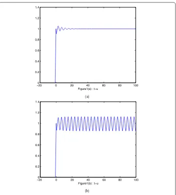
Figure 1The numerical solution of Eq. (2.11) with PD control Euler method corresponding to kp= 0.09,kd= 0.2 when (a)τ= 2.5, (b)τ= 3.5
Proof Assignq∗satisfiesATq∗=zq∗withz=e–iw∗0. Then there are
⎧ ⎪ ⎪ ⎨ ⎪ ⎪ ⎩ ˜
a0q∗0+q∗1=e–iw ∗ 0q∗
0,
q∗k=e–iw∗0q∗
k–1, k= 2, 3, . . . ,m,
˜
a1q∗0=e–iw ∗ 0q∗
m.
(4.5)
Letq∗m=a˜1eiw ∗
0K, by the normalizationq∗,q= 1 and direct computation, the lemma
fol-lows.
LetTcenterdenote a real eigenspace corresponding toe±iw ∗
0, which is two-dimensional
and is spanned by{(q),Im(q)¯ }, and letTstablebe a real eigenspace corresponding to all eigenvalues ofAT, other thane±iw∗0, which is (m– 1)-dimensional.
All vectorsx∈Rm+1can be decomposed as
(a)
(b)
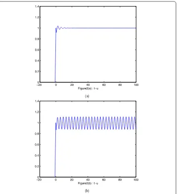
Figure 2The numerical solution of Eq. (2.11) with PD control Euler method corresponding tokp= 0,kd= 0 when (a)τ= 3, (b)τ= 5
wherev∈C,vq+v¯q¯∈Tcenter, andy∈Tstable. The complex variablevcan be viewed as a new coordinate onTcenter, so we have
v=q∗,x,
y=x–q∗,xq–q∗,xq.
Leta(λ) be a characteristic polynomial ofAandλ0=eiw ∗
0. Following the algorithms in [17]
and using a computation process similar to that in [15,19], we have
g20=
q∗,B(q,q),
g11=
q∗,B(q,q),
g02=
q∗,B(q,q),
g21=
q∗,B(q,w20)
+ 2q∗,B(q,w11)
(a)
(b)
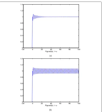
Figure 3The numerical solution of Eq. (2.11) with PD control Euler method corresponding to kp= –0.2,kd= 0.2 when (a)τ= 5, (b)τ= 7
where
w20= b0(q,q)
a(λ2 0)
pλ20–q
∗,B(q,q) λ20–λ0
q–q
∗,B(q,q)
λ20–λ0 q,
w11= b0(q,q)
a(1) p(1) –
q∗,B(q,q) 1 –λ0
q–q
∗,B(q,q)
1 –λ0 q.
So, we can get an expression for the critical coefficientc1(τ0∗)
c1
τ0∗=g20g11(1 – 2λ0) 2(λ20–λ0)
+ |g11| 2
1 –λ0
+ |g02| 2
2(λ20–λ0) +g21
2 . (4.6)
By (4.1), (4.2), and Lemma6, we get
c1
τ0∗=K 2
b2 a(e2w∗0i)
+ 2b 2
a(1)+c
(a)
(b)
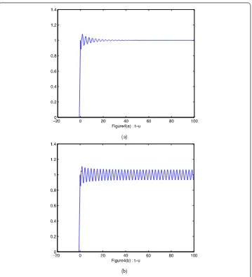
Figure 4The numerical solution of Eq. (2.11) with PD control Euler method corresponding to kp= –0.2,kd= –0.2 when (a)τ= 7, (b)τ= 10
We obtain the stability of the closed invariant curve by applying the Neimark–Sacker bifurcation theorem [20]. The results are as follows.
Theorem 3 If γβ > k nγ
p+(n–2)γ, here kd< 1, (2 –n)γ <kp < 0,or0 <kp<γ,then u=u∗ is
asymptotically stable for anyτ ∈[0,τ0∗)and unstable forτ >τ0∗.An attracting(repelling) invariant closed curve exists forτ>τ0∗if[e–iw0c
1(τ0∗)] < 0 (> 0). (When kp= 0,kd= 0,we obtain the results of the uncontrolled system.)
Remark2 The proportional control parameterkpand the derivative control parameterkd could decide the dynamics of system (3.2), e.g., the stability, the amplitude of the closed invariant curve, and the direction of the bifurcation [4,7,10,17,19].
5 Numerical simulations
(a)
(b)
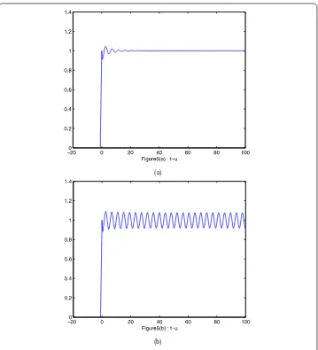
Figure 5The numerical solution of Eq. (2.11) with PD control Euler method corresponding to kp= 0.09,kd= 0.8 when (a)τ= 0.6, (b)τ= 0.8
Table 1 The values ofτ0of the PD control Euler method
kd 0.2 0 0.2 –0.2 0.8
kp 0.09 0 –0.2 –0.2 0.09
τ0 3.0317 4.3769 6.0871 9.1305 0.7579
Letβ= 0.2,γ = 0.1,n= 10, thenu∗= 1. From Table1we can see the different values of τ0by choosingkp,kdwith the PD control Euler method. Forh= 1/10, at differentkp,kd,
the results are shown in Figs.1–5.
From Figs.3and4and Table1, we could argue that the PD control Euler method enlarges the stable region by choosing control parameterskp< 0,kd< 1. From Figs.1and5, we could obtain that the PD control Euler method narrows the stable region by choosing control parameterskp> 0,kd< 1.
andkd= 0.8 (Fig.5). The results show that the derivative controller can significantly im-prove the speed of response of a control system.
6 Conclusions
In this paper, the problem of a proportional-derivative (PD) feedback numerical control method for Mackey–Glass system has been studied. In Sect.2, for DDE of Mackey–Glass system with PD controller, we analyzed the local stability of equilibria and existence of the Hopf bifurcation. In Sects.3and4, the PD control numerical strategy can delay (or ad-vance) the onset of an inherent bifurcation. Some computer simulations were performed to illustrate the theoretical results. According to the theoretical and numerical analysis, by choosing a different proportional control parameterkpand a derivative control param-eterkd, we can enlarge (or narrow) the stable region and postpone (or advance) the onset of the Neimark–Sacker bifurcation. PD control laws proved effective since they made the control system fairly sensitive to the parameter. In our future work, we intend to widen the application scopes of our theories.
Acknowledgements
The author is grateful to the referees for their helpful comments and constructive suggestions.
Funding
This work was supported by the Fundamental Research Funds for the Central Universities of China (16CX02055A) and by the National Natural Science Foundation of China (11401586, 11801566).
Competing interests
The authors declare that they have no competing interests.
Authors’ contributions
The authors declare that the study was realized in collaboration with the same responsibility. All authors read and approved the final manuscript.
Publisher’s Note
Springer Nature remains neutral with regard to jurisdictional claims in published maps and institutional affiliations.
Received: 28 July 2018 Accepted: 28 October 2018
References
1. Mackey, M.C., Glass, L.: Oscillations and chaos in physiological control systems. Science197, 287–289 (1977) 2. Yu, P., Chen, G.R.: Hopf bifurcation control using nonlinear feedback with polynomial functions. Int. J. Bifurc. Chaos14,
1683–1704 (2004)
3. Yu, P., Lü, J.H.: Bifurcation control for a class of Lorenz-like systems. Int. J. Bifurc. Chaos21, 2647–2664 (2011) 4. Chen, G.R., Moiola, J.L., Wang, H.O.: Bifurcation control: theories, methods, and applications. Int. J. Bifurc. Chaos10,
511–548 (2000)
5. Hill, D.J., Hiskens, I.A., Wang, Y.: Robust, adaptive or nonlinear control for modern power systems. In: Proceedings of the 32nd IEEE Conference on Decision and Control, San Antonio, TX, pp. 2335–2340 (1993)
6. Chen, Z., Yu, P.: Hopf bifurcation control for an Internet congestion model. Int. J. Bifurc. Chaos15, 2643–2651 (2005) 7. Ding, Y.T., Jiang, W.H., Wang, H.B.: Delayed feedback control and bifurcation analysis of Rossler chaotic system.
Nonlinear Dyn.61, 707–715 (2010)
8. Cheng, Z.S., Cao, J.D.: Hybrid control of Hopf bifurcation in complex networks with delays. Neurocomputing131, 164–170 (2014)
9. Su, H., Mao, X.R., Li, W.X.: Hopf bifurcation control for a class of delay differential systems with discrete-time delayed feedback controller. Chaos26(11), 113120 (2016)
10. Aström, K.J., Hägglund, T.: Advanced PID Control, ISA—The Instrumentation, Systems and Automation Society. Research Triangle Park, North Carolina (2006)
11. Rong, L.N., Shen, H.: Distributed PD-type protocol based containment control of multi-agent systems with input delays. J. Franklin Inst.352, 3600–3611 (2015)
12. Zhusubaliyev, Z.T., Medvedev, A., Silva, M.M.: Bifurcation analysis of PID-controlled neuromuscular blockade in closed-loop anesthesia. J. Process Control25, 152–163 (2014)
13. Ding, D.W., Zhang, X.Y., Cao, J.D., Wang, N., Liang, D.: Bifurcation control of complex networks model via PD controller. Neurocomputing175, 1–9 (2016)
15. Wulf, V., Ford, N.J.: Numerical Hopf bifurcation for a class of delay differential equation. J. Comput. Appl. Math.115, 601–616 (2000)
16. Ruan, S.G., Wei, J.J.: On the zeros of transcendental functions with applications to stability of delay differential equations with two delays. Dyn. Contin. Discrete Impuls. Syst., Ser. A Math. Anal.10, 863–874 (2003) 17. Kuznetsov, Y.A.: Elements of Applied Bifurcation Theory. Springer, New York (1995)
18. Hale, J.K.: Theory of Functional Differential Equations. Springer, Berlin (1977)
19. Wulf, V.: Numerical Analysis of Delay Differential Equations Undergoing a Hopf Bifurcation. University of Liverpool, Liverpool (1999)