Error estimates for an augmented method for one dimensional elliptic interface problems

(1)

R E S E A R C H

Open Access

Error estimates for an augmented method

for one-dimensional elliptic interface

problems

Qian Zhang

1*

_{, Zhifeng Weng}

2

_{, Haifeng Ji}

3

_{and Bin Zhang}

4

*_{Correspondence:}

[email protected] 1_{Institute of Information}

Technology, Nanjing University of Chinese Medicine, Nanjing, China Full list of author information is available at the end of the article

Abstract

Elliptic interface problems have many important scientific and engineering applications. Interface problems are encountered when the computational domain involves multi-materials with different conductivities, densities, or permeability. The solution or its gradient often has a jump across the interface due to discontinuous coefficients or singular sources. In this paper, optimal convergence of an augmented method is derived for one-dimensional interface problems. The dependence of the discontinuous coefficient in the error analysis is also considered. Numerical examples are presented to confirm the theoretical analysis and show that the estimate is sharp.

MSC: 65N15; 65N30; 35J60

Keywords: Interface problem; Immersed ﬁnite element; Augmented variable

1 Introduction

In scientific computation, we often encounter interface problems when multi-materials with different conductivities, densities, or permeability are involved. The solution or its gradient of the governing partial differential equation is often discontinuous due to dis-continuous coefficients or singular sources across the interface. Traditional numerical methods can not achieve optimal convergence unless the used mesh fits the interface. The methods using fitted meshes are often called fitted mesh methods. There are many fitted mesh methods in the literature (see, for example, [2,3,10]). However, the fitted mesh is dependent on the shape and the location of the interface. It may be difficult and time con-suming to generate a fitted mesh for a complicated interface. The difficulty becomes even severer for three-dimensional problems. Another disadvantage of the fitted mesh is en-countered when solving moving interface problems. Since the interface is moving, a new fitted mesh has to be generated at each time step and an interpolation is required to trans-fer the numerical solutions solved on different meshes. From this point of view, it would be preferable to use an unfitted mesh in which the interface can be arbitrarily located with respect to the fixed background mesh. Note that many other methods [4,18,20,21] can be used with fitted meshes when the problem is viewed as a problem with discontinuous co-efficients. For unfitted mesh methods, the difficulty is that the interface can pass through the interior of elements of the mesh. Thus, special treatment needs to be done on these elements.

(2)

There are many unfitted mesh methods in the literature, for instance, the extended fi-nite element method [5], the unfitted Nitsche’s finite element method [6], the immersed interface method [9,13], the immersed finite element/volume method [1,7,12,16,17,19] and the augmented finite difference/element method [8,11,14,15]. The extended finite element method (XFEM) enriches standard finite element space by adding extra func-tions near the interface to treat the jumps of the exact solution. The degrees of freedom of the XFEM often change with moving interfaces. In the unfitted Nitsche’s finite element method, the function in finite element spaces is discontinuous across the interface and the interface conditions are absorbed in the bilinear form. A penalty is also added into the bi-linear form to deal with the discontinuous of the finite element functions. The immersed finite element methods (IFEMs) are a class of unfitted mesh methods that modify the basis function on interface elements according to the interface conditions to capture the jumps of the exact solution. The bilinear form and the degrees of freedom are the same as if there was no interface. If the coefficient is a constant without jumps, then the stiffness matrix is the same as that obtained by traditional finite element for the problem without interfaces. And only the right-hand side needs to be modified according to the interface conditions. The augmented method is developed based on the above observations. In the augmented method, an augmented variable is introduced along the interface so that the original in-terface problem can be transferred to a new inin-terface problem without discontinuous co-efficients. Thus, the efficient method can be used by only modifying the right-hand side. The augmented variable should be chosen such that the original interface conditions are satisfied. Extensive numerical examples in [8] show that the augmented method achieves optimal convergence in theL2_,_H1 _and_L∞ _{norms. In this work, we derive the optimal}

error estimates for the augmented method for one-dimensional interface problems. The dependence of the discontinuous coeﬃcient is included. Numerical results show that the estimate is sharp.

The rest of the paper is organized as follows. In Sect.2, we describe the model prob-lem and some preliminaries. We choose the augmented variable and rewrite the inter-face problem. In Sect.3, we analyze the method for interface problems only with singular sources where the augmented variable is assumed to be given. The augmented method and the error estimates are provided in Sect.4. Finally, some numerical examples are pre-sented in Sect.5to conﬁrm the theoretical analysis.

2 Preliminaries

Let= (a,b) be a ﬁnite interval. Assume that the domainis separated into two sub-domains1= (a,α) and2= (α,b) by an interface pointα∈. Consider the following

one-dimensional second-order interface problem:

⎧ ⎨ ⎩

–(β(x)u(x))=f(x), x∈1∪2,

u(a) =u(b) = 0, (2.1)

where the diffusion coefficientβ(x) is assumed to have a finite jump across the interfaceα. We also assume that the coefficientβ(x) > 0 is a piecewise constant, i.e.,

β(x) =

⎧ ⎨ ⎩

β1, x∈1,

β2, x∈2.

(3)

At the interfaceα, the solution is assumed to satisfy the interface conditions

The augmented variablegshould be chosen such that the augmented equation

s

The augmented method is to discretize (2.5) and (2.6), respectively. In the next section, we present the method to discretize (2.5) and give corresponding error analysis. The dis-cretization of (2.6) is discussed in Sect.4.

3 The method for interface problems only with singular sources

(4)

Leta=x0<x1<· · ·<xk<xk+1<· · ·<xN =b be a partition of [a,b] independent of

the interface pointα. Assume that there exists a numberksuch thatα∈[xk,xk+1). We

call the element [xk,xk+1] the interface element. The rest of the elements [xi,xi+1],i=kare

called non-interface elements. Leth:=max0≤i≤N–1(xi+1–xi). We assume that the partition

is quasi-uniform, i.e., there exists a generic constantCindependent ofhsuch thath≤ Cmin₀_≤_i_≤_N_–1(xi+1–xi).

LetVL

h be the usual conforming linear ﬁnite element space which is deﬁned as

V_hL= vh∈C0(a,b)|vh(x) is linear on [xk,xk+1]

for 0≤k≤N– 1,vh(a) =vh(b) = 0

. (3.2)

We also deﬁne the standard nodal interpolation operatorIL h by

I_hLu∈V_hL, I_hLu(xi) =u(xi), i= 0, 1, . . . ,N. (3.3)

Deﬁne

χ(x) =

⎧ ⎨ ⎩

1, x>α,

0, x≤α, and ue(x) = (x–α)q+g. (3.4) Thus, we can deﬁne

uJ_h(x) =u–I_hLu, whereu(x) =χ(x)ue(x). (3.5)

By the deﬁnition, we conclude that

u(x) =

⎧ ⎨ ⎩

(x–α)q+g, x>α,

0, x≤α, and JuKα=g,

q

(u)y_α=q.

It is easy to verify that

uJ_h(x) = 0, x∈[a,xk]∪[xk+1,b], (3.6)

and

uJ_h(x)= 0, x∈(xk,xk+1), q

uJ_hy_α=g, quJ_hy_α=q. (3.7) The immersed ﬁnite element (IFE) spaceV_hJis deﬁned by

V_hJ= vh∈L2(a,b)|vh=vLh+uJh,v L h∈VhL

. (3.8)

The method for the interface problem (2.5) is: ﬁnduh∈VhJsuch that

uh=uLh+uJh,

auL h,vh

= (f,vh) –qvh(α) –a

uJ_h,vh

, ∀vh∈vLh.

(3.9)

(5)

Lemma 3.1 There exists a generic constant C> 0independent of h,αandβsuch that

θ∈W2,∞(a,b). Using the standard interpolation error estimate, we obtain

I_hLθ–θ

(6)

On the interface element (xk,xk+1), we have xk+1

xk

u–I_hLu–u_hJ(vh)dx

= (vh)

α

xk

u–I_hLu–uJ_hdx+

xk+1

α

u–I_hLu–uJ_hdx

= (vh)

u–I_hLu–uJ_hα_x k+

u–I_hLu–uJ_hx_αk+1

= (vh)

–JuKα+

q

I_hLuy_α+quJ_hy_α= 0. (3.18)

Then we have

auL_h–I_hLu,vh

= 0. (3.19)

Takingvh=uL_h–I_hLu, we conclude that

auL_h–I_hLu,uL_h–I_hLu= 0, (3.20)

which implies that

uL_h=I_hLu. (3.21)

Thus,

uh–u=uLh+u J

h–u=IhLu+u J

h–u, (3.22)

which, together with Lemma3.1, completes the proof. Next, we consider that the augmented variable is given with errors, i.e.,G=g+E(G). Then, by the method (3.9), we need to replacegbyGin (3.4). Now the functionuJ_hbecomes

U_hJ and the numerical solution of the method is

Uh=UhL+U J

h. (3.23)

Theorem 3.3 Assuming the augmented variable is given with the errorE(G) =G–g,then there exists a generic constant C> 0independent of h,αandβsuch that

Uh–uL∞(a,b)≤Ch2u_L∞₍1∪2)+ 2E(G). (3.24)

Proof Obviously, we have

uJ_h–U_hJ= –χ(x)E(G)+I_hLχ(x)E(G) (3.25)

and

auL_h–U_hL,vh

= –auJ_h–U_hJ,vh

(7)

From (3.25), we get

the solution is the well-known Green’s functionG(x;xi), which is deﬁned as

(8)

Thus, we obtain

uL_h–U_hL_L∞₍_a_,_b₎≤E(G).

Using (3.28), (3.34) and Theorem (3.2), we get

Uh–uL∞(a,b)≤ uh–uL∞(a,b)+Uh–uhL∞(a,b)

≤ uh–uL∞(a,b)+UhL–uLhL∞(a,b)+U

J h–u

J hL∞(a,b)

≤Ch2u_L∞₍1∪2)+ 2E(G), (3.35)

which completes the proof.

4 Augmented method for discontinuous coefﬁcients and error estimates

In continuous cases, the augmented variablegneeds to be chosen such that the interface condition (2.6) is satisﬁed. In the augmented method, the numerical augmented variable

Gshould be chosen such that

s

Uh β

{

α

=Uh(α

+₎

β2

–Uh(α

–₎

β1

=w, (4.1)

whereUh(see (3.23)) is the solution of method for (3.9) withgreplaced byG. Note that

(4.1) is a discretization of the augmented equation (2.6).

The matrix-vector form of (3.9) and (4.1) can be written as (see [8])

A B

E H

Uh

G

=

F1

F2

. (4.2)

EliminatingUhfrom (4.2), we get the Schur complement system forG

H–EA–1BG=F2–EA–1F1. (4.3)

To simplify the notation, we denote the Schur complement system by

SG=F, whereS=H–EA–1B,F=F2–EA–1F1.

For one-dimensional problems, the Schur complementSis a number. Note that the ma-trices such asA,B,E,Hare not formed explicitly in implementations and are only used for theoretical analysis.

Deﬁne the truncation error of the augmented equation by

T:=SE(G)=S(G–g) =SG–Sg. (4.4)

(9)

Lemma 4.1 We have

Then, using Theorem3.2, we conclude

|T|=SE(G)=S(G–g)≤C

which completes the proof of this lemma. Given a guess augmented variableG0_{, the residual of the Schur complement is deﬁned}

as

Next, we show that the Schur complement satisfying|S|is independent of the mesh size

hand|S| = 0.

h be the solution of the method (3.9) with the augmented

(10)

augmented variable given asg= 1. From (4.8), we have

It is easy to check that the exact solution is

ψ(x) =

Using the result (3.21), which is proved in Theorem3.2, we have

uL_h,1–uL_h,0=IL_hψ. (4.15)

(11)

Theorem 4.3 Let G and Uhbe the solution of the augmented method(3.9)and(4.1).There

exists a constant C> 0independent of h,αandβsuch that |G–g| ≤C 1

min{k1,k2}

h2u_L∞₍1∪2), (4.18)

and

Uh–uL∞(a,b)≤C

1

min{k1,k2}

h2u_L∞₍₁_∪₂₎, (4.19)

where k1= (b–α)/(b–a) > 0,k2= (α–a)/(b–a).

Proof Using Lemma4.2and Lemma4.1, we have

_E(G)=|G–g|=S–1T≤C β1+β2 k1β1+k2β2

h2u_L∞₍₁_∪₂₎. (4.20)

Note thatk1> 0,k2> 0,k1+k2= 1 andβ(x) > 0. Ifβ2≥β1, then we get

β1+β2

k1β1+k2β2 ≤

2β2

β2k2

= 2

k2

. (4.21)

Ifβ1>β2, then we have

β1+β2

k1β1+k2β2 ≤

2β1

β1k1

= 2

k1

. (4.22)

Thus,

_E₍_G₎_≤_C 1

min{k1,k2}

h2u_L∞₍₁_∪₂₎, (4.23)

which, together with Theorem3.3completes the proof of this theorem.

Remark4.4 The numerical solution of the original interface problem (2.1)–(2.3) isUh=

Uh/β. We have

Uh–uL∞(a,b)≤C

1

min{β1,β2}

1

min{k1,k2}

h2u_L∞₍1∪2)

≤C 1 min{β1,β2}

1

min{k1,k2}

h2fL∞(1∪2), (4.24)

where we have used the fact –u=f in the last inequality.

5 Numerical examples

In this section, we present numerical examples to conﬁrm our theoretical results. In the following examples, we consider an unit interval [0, 1] with uniform partitions. The inter-face point is given asα=π/10.

Leteh=u–Uh. The method achieves convergence orderrif we can showehL∞≈Chr.

(12)

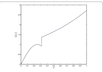
Figure 1The exact solution of Example1

x=logh. For the interface problem, the constantCdepends on the relative location of the interface and the mesh. Thus, we compute the slope of least squares ﬁtting which can be regarded as the average convergence order.

Example1 The analytic solutionu(x) is given as

u(x) =

⎧ ⎨ ⎩

sin(2πx), 0≤x<α,

ex_, _α_<_x_≤_1.

Thus, the corresponding jump conditions are

JuKα=eα–sin(2π α),

q

βuy_α=β2eα– 2πβ1cos(2π α).

We considerβ1= 1,β2= 5 in this example. The exact solution is shown in Fig.1. Numerical

results are reported in Fig.2. We can see that the augmented method achieves optimal convergence.

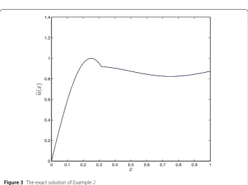
Example2 The analytic solutionu(x) is given as

u(x) =

⎧ ⎨ ⎩

sin(2πx)/β1, 0≤x<α,

sin(2πx)/β2– (1/β2– 1/β1)sin(2π α), α<x≤1.

Thus, we have

JuKα= 0,

q

(13)

Figure 2Numerical results obtained by the augmented method for Example1withβ1= 1 andβ2= 5

Figure 3The exact solution of Example2

which are homogeneous jump conditions. We considerβ1= 1,β2= 20 in this example.

The corresponding source function is

f(x) = 4π2sin(2πx), 0 <x< 1.

(14)

Figure 4Numerical results obtained by the augmented method for Example2withβ1= 1 andβ2= 20

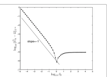
Figure 5Numerical results obtained by the augmented method for Example2withβ1= 1,N= 512

Next, we consider the dependence of the discontinuous coeﬃcient β. We solve the problem withβ1= 1 and varyingβ2. Errors are obtained by the augmented method with

N= 512. Note thatfL∞(1∪2)= 4π2is independent ofβin this example. Ifβ2≤1, then

the error should beO(β₂–1) according to the estimate (4.24). Ifβ2≥1, then the error should

(15)

6 Conclusion

This article gives rigorous error estimates for the augmented method for one-dimensional interface problems. The inﬂuence of the discontinuous coeﬃcient and the location of the interface is considered in the error estimation. Numerical results show that the estimate is sharp. In future work, we will extend the results to high-dimensional interface problems.

Acknowledgements

The authors would like to thank the referees for their useful comments, which improved the quality of this paper.

Funding

This work was partially supported by the Natural Science Foundation of the Jiangsu Higher Education Institutions of China (Grant No. 17KJB110014), the open project program of Jiangsu Key Laboratory for NSLSCS (Grant No. 201704), the National Natural Science Foundation of China (Grant Nos. 11701291 and 11701197), and the Natural Science Foundation of Jiangsu Province (Grant No. BK20160880).

Availability of data and materials Not applicable.

Competing interests

The authors declare that they have no competing interests.

Authors’ contributions

All authors read and approved the ﬁnal manuscript.

Author details

1_{Institute of Information Technology, Nanjing University of Chinese Medicine, Nanjing, China.}2_{Fujian Province University}

Key Laboratory of Computation Science, School of Mathematical Sciences, Huaqiao University, Quanzhou, China.3_School of Science, Nanjing University of Posts and Telecommunications, Nanjing, China.4_{School of Mathematical Sciences, Qufu} Normal University, Qufu, China.

Publisher’s Note

Springer Nature remains neutral with regard to jurisdictional claims in published maps and institutional aﬃliations.

Received: 11 May 2018 Accepted: 21 August 2018

References

1. An, N., Chen, H.: A partially penalty immersed interface ﬁnite element method for anisotropic elliptic interface problems. Numer. Methods Partial Diﬀer. Equ.30, 1984–2028 (2014)

2. Bramble, J.H., King, J.T.: A ﬁnite element method for interface problems in domains with smooth boundaries and interfaces. Adv. Comput. Math.6, 109–138 (1996)

3. Chen, Z., Zou, J.: Finite element methods and their convergence for elliptic and parabolic interface problems. Numer. Math.79, 175–202 (1998)

4. Feng, Q., Meng, F., Zhang, Y.: Some new finite difference inequalities arising in the theory of difference equations. Adv. Differ. Equ.2011, 21 (2011)

5. Fries, T., Belytschko, T.: The extended/generalized ﬁnite element method: an overview of the method and its applications. Int. J. Numer. Methods Eng.84, 253–304 (2010)

6. Hansbo, A., Hansbo, P.: An unﬁtted ﬁnite element method, based on Nitsche’s method, for elliptic interface problems. Comput. Methods Appl. Mech. Eng.191, 5537–5552 (2002)

7. He, X., Lin, T., Lin, Y.: The convergence of the bilinear and linear immersed ﬁnite element solutions to interface problems. Numer. Methods Partial Diﬀer. Equ.28, 312–330 (2012)

8. Ji, H., Chen, J., Li, Z.: A new augmented immersed ﬁnite element method without using SVD interpolations. Numer. Algorithms71, 395–416 (2016)

9. LeVeque, R., Li, Z.: The immersed interface method for elliptic equations with discontinuous coeﬃcients and singular sources. SIAM J. Numer. Anal.31, 1019–1044 (1994)

10. Li, J., Markus, J., Wohlmuth, B., Zou, J.: Optimal a priori estimates for higher order ﬁnite elements for elliptic interface problems. Appl. Numer. Math.60, 19–37 (2010)

11. Li, Z.: A fast iterative algorithm for elliptic interface problems. SIAM J. Numer. Anal.35, 230–254 (1998)

12. Li, Z.: The immersed interface method using a ﬁnite element formulation. Appl. Numer. Math.27, 253–267 (1998) 13. Li, Z., Ito, K.: The Immersed Interface Method: Numerical Solutions of PDEs Involving Interfaces and Irregular

Domains. Frontiers in Applied Mathematics, vol. 33. SIAM, Philadelphia (2006)

14. Li, Z., Ji, H., Chen, X.: Accurate solution and gradient computation for elliptic interface problems with variable coeﬃcients. SIAM J. Numer. Anal.55(2), 570–597 (2017)

15. Li, Z., Lai, M., Peng, X., Zhang, Z.: A least squares augmented immersed interface method for solving Navier–Stokes and Darcy coupling equations. Comput. Fluids167, 384–399 (2018)

(16)

17. Lin, T., Lin, Y., Zhang, X.: Partially penalized immersed ﬁnite element methods for elliptic interface problems. SIAM J. Numer. Anal.53, 1121–1144 (2015)

18. Liu, W., Cui, J., Xin, J.: A block-centered ﬁnite diﬀerence method for an unsteady asymptotic coupled model in fractured media aquifer system. J. Comput. Appl. Math.337, 319–340 (2018)

19. Oevermann, M., Klein, R.: A Cartesian grid ﬁnite volume method for elliptic equations with variable coeﬃcients and embedded interfaces. J. Comput. Phys.219, 749–769 (2006)

20. Wang, B., Meng, F., Fang, Y.: Eﬃcient implementation of RKN-type Fourier collocation methods for second-order diﬀerential equations. Appl. Numer. Math.119, 164–178 (2017)