R E S E A R C H
Open Access
Dynamics of a delayed SEIQ epidemic
model
Wanjun Xia
1*, Soumen Kundu
2and Sarit Maitra
2*Correspondence:
1School of Management Science
and Engineering, Anhui University of Finance and Economics, Bengbu, China
Full list of author information is available at the end of the article
Abstract
In this work we consider an epidemic model that contains four species susceptible, exposed, infected and quarantined. With this model, first we find a feasible region which is invariant and where the solutions of our model are positive. Then the persistence of the model and sufficient conditions associated with extinction of infection population are discussed. To show that the system is locally asymptotically stable, a Lyapunov functional is constructed. After that, taking the delay as the key parameter, the conditions for local stability and Hopf bifurcation are derived. Further, we estimate the properties for the direction of the Hopf bifurcation and stability of the periodic solutions. Finally, some numerical simulations are presented to support our analytical results.
Keywords: SEIQ model; Delay; Boundedness; Lyapunov functional; Persistence; Hopf bifurcation; Periodic solution
1 Introduction
Since the principles to the mathematical model of epidemics, as the susceptible–infected– susceptible (SIS) model and the susceptible–infected–removed (SIR) model, were pre-sented in [1, 2], the mathematical investigation of disease transmission has developed quickly. As is well known, many epidemic diseases such as HIV/AIDS [3], H1N1 [4], H5N1 [5] and SARS [6], are harmful to individual health and to the stability of our society. It is an increasingly urgent issue to control the prevalence of epidemic diseases. Mathemat-ical epidemiology, which describes the prevalence of epidemic diseases by building and analyzing mathematical models, has been one of the major areas of biology. In recent years, mathematical models have become one of the important tools in the investiga-tion of the prevalence and control of epidemic diseases since the pioneering work of Ker-mack and Mckendrick [7,8]. For example, the SIRS (Susceptible–Infectious–Recovered– Susceptible) epidemic model [9–12], the SEIS (Susceptible–Exposed–Infectious–Suscept-ible) epidemic model [13–16], SEIR (Susceptible–Exposed–Infectious–Recovered) epi-demic model [17–20], the SEIRS (Susceptible–Exposed–Infectious–Recovered–Suscept-ible) epidemic model [21–25] and epidemic models with vaccination [26–28].
In real world, some people can be quarantined once they are found to have been infected with epidemic diseases in the exposed state or the infectious state. Based on this
Table 1 Parameters and their meanings in this paper
Parameter Description
A the constant recruitment rate of the population
β The infection rate of the susceptible population
μ The natural mortality rate of all populations
c The rate that the infected recovers and comes into the susceptible class
ε The rate at which some exposed people become infective
α The mortality rate of the infected and quarantined population due to disease
σ1 The quarantined rate of the exposed population
σ2 The quarantined rate of the infected population
γ1 The recovery rate of the exposed population
γ2 The recovery rate of the infected population
γ3 The recovery rate of the quarantined population
ation, recently, Chen et al. [29] proposed the following epidemic model with quarantine:
⎧ ⎪ ⎪ ⎪ ⎪ ⎪ ⎪ ⎨ ⎪ ⎪ ⎪ ⎪ ⎪ ⎪ ⎩
dS(t)
dt =A–βS(t)I(t) –μS(t) +cI(t), dE(t)
dt =βS(t)I(t) – (μ+ε+σ1+γ1)E(t), dI(t)
dt =εE(t) – (μ+α+c+σ2+γ2)I(t), dQ(t)
dt =σ1E(t) +σ2I(t) – (μ+α+γ3)Q(t),
(1)
whereS(t),E(t),I(t) andQ(t) are the numbers of the susceptible, the exposed, the infected and the quarantined individuals at timet, respectively. The meanings of the parameters are listed in Table1.
With this model they [29] investigated the local and the global stability of system (1), and they also estimated the domain of attraction of system (1).
the latent delay into system (1) and study the following delayed system:
⎧ ⎪ ⎪ ⎪ ⎪ ⎪ ⎪ ⎨ ⎪ ⎪ ⎪ ⎪ ⎪ ⎪ ⎩
dS(t)
dt =A–βS(t)I(t) –μS(t) +cI(t), dE(t)
dt =βS(t)I(t) – (μ+σ1+γ1)E(t) –εE(t–τ), dI(t)
dt =εE(t–τ) – (μ+α+c+σ2+γ2)I(t), dQ(t)
dt =σ1E(t) +σ2I(t) – (μ+α+γ3)Q(t),
(2)
subject to the initial conditions
S(θ) =φ1(θ) > 0,
E(θ) =φ2(θ) > 0,
I(θ) =φ3(θ) > 0,
Q(θ) =φ4(θ) > 0, θ∈[–τ, 0),φi(0) > 0,i= 1, 2, 3, 4,
(3)
where the meanings of the parameters are given in Table1and they are assumed to be positive andτ is the latent delay of the disease.
The organization of the paper is as follows. In the next section, it is shown that the so-lution of (2) is positive and bounded in a feasible regionR¯, which is invariant. Also, the persistence of the proposed model and some sufficient conditions associated with extinc-tion of infective populaextinc-tion are discussed. In Sect.3, the condition for local asymptotical stability is examined by constructing a suitable Lyapunov functional. By taking the latent delayτ as the bifurcation parameter, the conditions for the occurrence of Hopf bifurca-tion are derived in Sect.4. Further, the direction of Hopf bifurcation and the stability of the periodic solution are examined in Sect.5. Some numerical results are carried out for our expository results in Sect.6. Finally, the paper ends with the conclusion of the work.
2 The boundedness, persistence and extinction of infected population
2.1 The boundedness
In this section we shall discuss about the positivity and boundedness of solution of system (2).
For this purpose, we assume the functionVto be
V(t) =S(t) +E(t) +I(t) +Q(t). (4)
Taking the derivative of (4) and using (2) we get
˙
V(t) =A–μS(t) – (μ+γ1)E(t) – (μ+α+γ2)I(t) – (μ+α+γ3)Q(t), (5)
whereS(t) > 0 andE(t),I(t),Q(t)≥0.
IfE(t) = 0,I(t) = 0 andQ(t) = 0 from (5) we get
lim
t→∞supV(t)≤
A
Also, ifV(t) >Aμ thenV˙(t) < 0. Therefore, we get 0 <V≤ Aμ, i.e., we get a feasible re-gionR¯:
¯
R=S(t),E(t),I(t),Q(t)∈R4: 0 <S(t) +E(t) +I(t) +Q(t)≤A
μ .
Thus we see that the solution of system (2) is bounded and independent of the initial condition. So the feasible regionR¯is an invariant set. Also, asA> 0,μ> 0,μA> 0, i.e., the feasible regionR¯ is positive.
Hence all solutions of (2) will enter the fieldR¯and will remain inR¯.
2.2 The persistence and extinction of infection species
In this section, we will consider the ultimate state of infection, that is, the disease will be either persistent or extinct ultimately.
Since the variable Qdoes not appear explicitly in the first three equations in system (2), we need only to consider the dynamics of a subsystem consisting of the first three equations in system (2). We have
dS(t)
dt =A–βS(t)I(t) –μS(t) +cI(t), dE(t)
dt =βS(t)I(t) – (μ+σ1+γ1)E(t) –εE(t–τ), dI(t)
dt =εE(t–τ) – (μ+α+c+σ2+γ2)I(t),
(7)
From the first equation in system (7), we have ds dt ≤ μ(
A
μ – S); it implies that limt→∞supS(t)≤ Aμ; therefore, the setω={(S,E,I)∈R3+:S≤Aμ} is positively invariant under system (7). Thus, we only consider the dynamical behavior of system (7) on the setω.
WhenR0< 1, define the function
V1=ρE+I, (8)
whereρ∈(1 ε,
μ+α+c+σ2+γ2
β(A/μ) ), then the derivative ofV1with respect totalong the solution of (7) on the setωis given by
dV1
dt = –ρ(μ+σ1+γ1)E(t) + (1 –ρε)E(t–τ) +
ρβA
μ– (μ+α+c+σ2+γ2) I(t). (9)
Thus,
dV1
dt ≤(1 –ρε)E(t–τ) +
ρβA
μ– (μ+α+c+σ2+γ2) I(t). (10)
Asρ∈(1ε,μ+α+c+σ2+γ2
β(A/μ) ), we have 1 –ρε< 0, andρβ A
μ– (μ+α+c+σ2+γ2) < 0. Therefore we consider a positive numberσ, such that, 1 –ρε<σρ(R0– 1) and 1 –ρε< 0, andρβAμ– (μ+α+c+σ2+γ2) <σ(R0– 1). Thus from (10) we can write
V1(t)≤V1(0)exp
σ(R0– 1)t
whereV1(0) =ρE(0) +I(0), therefore forR0< 1 we have
lim
t→∞V1(t) = 0, i.e., t→∞limE(t) = 0 =t→∞limI(t).
This shows that the disease will extinct ifR0< 1.
In order to discuss the persistence of the disease, we first introduce some definitions; then we follow the steps in [41].
Assume thatXis a locally compact metric space with metricd, and letFbe a closed subset ofXwith boundaryδF and interiorintF. Letπ be a semidynamical system de-fined on F. We say thatπ is persistent if, for allu∈intF,limt→+∞infd(π(u,t),δF) > 0, and we say that π is uniformly persistent if there isξ > 0 such that, for all u∈intF, limt→+∞infd(π(u,t),δF) >ξ.
In [41], Fonda gives a result about persistence in terms of repellers. A subset of
F is said to be a uniform repeller if there is an η> 0 such that, for each u∈F \, limt→+∞infd(π(u,t),) >η. A semiflow on a closed subsetF of a locally compact met-ric space is uniformly persistent if the boundary ofFis repelling in a suitable strong sense.
Lemma 1 Letbe a compact subset of X such that X\is positively invariant.A neces-sary and sufficient condition forto be a uniform repeller is that there exist a neighborhood Uofand a continuous function P:X→R+satisfying
(1) P(u) = 0if and only ifu∈,
(2) for allu∈U\there is aTu> 0such thatP(π(u,Tu)) >P(u).
For anyu0= (S0,E0,I0)∈ω, there is a unique solutionπ(u0,t) = (S,E,I)(t;u0) of system (7), which is defined inR+and satisfiesπ(u0, 0) = (S0,E0,I0). Sinceωis a positively invariant set of system (7), thenπ(u0,t)∈ωfort∈R+and it is a semidynamical system inω. Here, we will prove that, when R0> 1,={(S,E,I)∈ :I= 0} is a uniform repeller, which implies that the semidynamical systemπis uniformly persistent. Obviously,I(t) > 0 for
t> 0 ifI(0) > 0, thenω\is invariant to (7). Again the setis a compact subset ofω. LetP:ω→R+be defined byP(S,E,I) =I, and let U ={(S,E,I)∈ω:P(S,E,I) <ζ1}, where
ζ1> 0 is small enough so that
A–μ(μ+σ1+γ1+ε)(μ+α+c+σ2+γ2)
βε
–
(μ+σ1+γ1+ε)(μ+α+c+σ2+γ2)
ε –c ζ1> 0. (12)
SinceR0> 1, the positive numberζ1is sufficiently small to satisfy the inequality (12). Assume that there isu¯∈U(u¯ = (S¯,E¯,I¯)) such that for eacht> 0 we haveP(π(u¯,t)) <
P(u¯) <ζ1, which implies thatI(t,u¯) <ζ1fort> 0. From the first equation of (7) we have
dS
dt ≥A+cζ1– (μ+βζ1)S, (13)
then
lim
t→∞infS(t,u¯)≥
A+cζ1
μ+βζ1
For sufficiently large number ofT> 0 we haveS(t,u¯) > A+cζ1
μ+βζ1 fort≥T.
Now we define another functionV2(t) = (1 –ζ2)E(t) +μ+σ1β+γ1+εI(t), whereζ2(0 <ζ2< 1) is a sufficiently small constant so that
A–μ(1 –ζ2)(μ+σ1+γ1+ε)(μ+α+c+σ2+γ2)
βε
>
(μ+σ1+γ1+ε)(μ+α+c+σ2+γ2)
ε –c ζ1. (15)
Now we differentiateV2(t) along withπ(u¯,t) as follows:
dV2
dt ≥
ζ2(μ+σ1+γ1)
β E(t) +
A–μ(1 –ζ2)(μ+σ1+γ1+ε)(μ+α+c+σ2+γ2)
βε
–
(μ+σ1+γ1+ε)(μ+α+c+σ2+γ2)
ε –c
ζ1 I(t), (16)
dV2
dt >κV2, (17)
where
κ=min
ζ2(μ+σ1+γ1)
β(1 –ζ2) ,
β μ+σ1+γ1
A–μ(1 –ζ2)(μ+σ1+γ1+ε)(μ+α+c+σ2+γ2)
βε
–
(μ+σ1+γ1+ε)(μ+α+c+σ2+γ2)
ε –c
ζ1 > 0.
Thus we see that
lim
t→∞V2(t) = +∞. (18)
Therefore, this proof shows that, for eachu∈ω\withubelonging to a suitable small neighborhood of, there is someTusuch thatP(π(u,Tu)) >P(u). Therefore, it follows
from Lemma1that={(S,E,I)∈:I= 0}is a uniform repeller whenR0> 1, i.e., the infection is uniformly persistent. So we conclude that system (7) will be persistent for
R0> 1 and infection will be extinct whenR0< 1.
3 Stability analysis
Based on the analysis in [29], we know that ifR0> 1, then system (2) has a unique endemic equilibriumP∗(S∗,E∗,I∗,Q∗), where
S∗= A
μR0
,I∗= εE
∗
μ+α+c+σ2+γ2 ,
E∗= A(R0– 1)(μ+α+c+σ2+γ2)
R0[(μ+σ1+γ1)(μ+α+c+σ2+γ2) +ε(μ+α+σ2+γ2)] ,
Q∗= (μ+α+c+σ2+γ2)σ1+εσ2 (μ+α+γ3)(μ+α+c+σ2+γ2)
R0=
Aβε
μ(μ+ε+σ1+γ1)(μ+α+c+σ2+γ2) .
In this section the linear stability of system (2) is discussed by constructing a suitable Lyapunov functional given in (20). For this purpose, letu1(t) =S(t) –S∗,u2(t) =E(t) –E∗,
Now following the steps in [42,43], we shall check the stability of the system by assuming a suitable Lyapunov functionw(v)(t) as follows:
w(u)(t) =k1w1(u)(t) +k2w2(u)(t) +k3w3(u)(t) +k4w4(u)(t) +k5w5(u)(t)
All the parameters are assumed to be positive and chosen in such a way thatk1> 0,
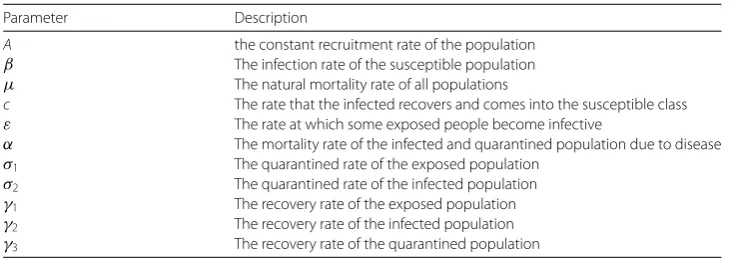
Figure 1 τversus1,2,3,4have been plotted, where all the1,2,3,4are negative for τ≤τ0= 13.9858
Figure 2 τversus1,2,3,4have been plotted, where all the1,2,3,4are positive and τ≥τ0= 13.9858
derivative of (20), and using (19) we get
d
dtw(u)(t)≤1u
2
1+2u22+3u23+4u24, (21)
where the expressions for1,2,3,4are given in theAppendix.
Theorem 1 If the value of the delayτ satisfy the conditions1< 0,2< 0,3< 0,4< 0
then the interior equilibrium point P∗(S∗,E∗,I∗,Q∗)of(2)is locally asymptotically stable
(Fig.1).Otherwise if any one of thei become positive then the system will be unstable
(Fig.2)
Proof Let=max{1,2,3,4}. Then, fort>T, from (21) we get
w(u)(t) +
t
T
fort≥T, impliesu2
1+u22+u23+u24∈L1[T,∞]. It is easy to conclude from (19) and the boundedness ofu(t) thatu2
1(t) +u22(t) +u23(t) +u24(t) is uniformly continuous. Using Bar-balat’s lemma [44], we can say that
lim t→∞
u21+u22+u23+u24= 0. (22)
So the internal solution of (19) and the solutions of (2) are asymptotically stable, i.e., the positive equilibriumP∗of (2) is locally asymptotically stable. Hence, this completes the
proof.
Remark As1,2,3,4depends on the delayτand the local stability condition forP∗ of system (2) is preserved for smallτ satisfying1< 0,2< 0,3< 0,4< 0. For a set of parameters,1,2,3,4have been plotted in Fig.1, it shows that all the values of
are negative within an interval ofτ, which implies the stability of the system. But, for increased values of the latent delayτ, all the values ofare positive (see Fig.2), which shows that the system is unstable.
4 Linear stability and Hopf-bifurcation analysis
Here we shall discuss the condition for linear stability and then takingτ as bifurcation parameter the condition for Hopf bifurcation is discussed. The characteristic equation of system (2) is
λ4+m3λ3+m2λ2+m1λ+m0+
n3λ3+n2λ2+n1λ+n0
e–λτ= 0, (23)
where
m0=a1a4a6a9,
m1= –
a1a4a6+a9(a1a4+a1a6+a4a6)
,
m2=a1a4+a1a6+a4a6+a9(a1+a4+a6),
m3= –(a1+a4+a6+a9),
n0=a1a9(a6b1–a5b2) +a2a3a9b2,
n1=a5b2(a1+a9) –a2a3b2–b1(a1a6+a1a9+a6a9),
n2=b1(a1+a6+a9) –a5b2, n3= –b1,
and
a1= –
βI∗+μ, a2=c–βS∗, a3=βI∗,
a4= –(μ+σ1+γ1), a5=βS∗,
a6= –(μ+α+c+σ2+γ2),
a7=σ1, a8=σ2,a9= –(μ+α+γ3), b1= –ε, b2=ε.
Theorem 2 For system(2),if R0> 1and the conditions(H1)–(H2)hold,then the endemic
undergoes a Hopf bifurcation at the endemic equilibrium P∗(S∗,E∗,I∗,Q∗)whenτ=τ0and
a family of periodic solutions bifurcate from the endemic equilibrium P∗(S∗,E∗,I∗,Q∗).The conditions(H1)and(H2)are described in the following.
Proof The proof proceeds by using some lemmas.
Lemma 2([29]) When R0> 1,the unique endemic equilibrium P∗(S∗,E∗,I∗,R∗)is locally
asymptotically stable whenτ= 0for system(2).
Forτ > 0, letλ=iω(ω> 0) be the root of Eq. (23), then ⎧
⎨ ⎩
(n1ω–n3ω3)sinτ ω+ (n0–n2ω2)cosτ ω=m2ω2–ω4–m0, (n1ω–n3ω3)cosτ ω– (n0–n2ω2)sinτ ω=m3ω3–m1ω,
(24)
which leads to
ω8+l3ω6+l2ω4+l1ω2+l0= 0, (25)
where
l0=m20–n20,
l1=m21– 2m0m2+ 2n0n2–n21,
l2=m22+ 2m0– 2m1m3–n22+ 2n1n3,
l3=m23–n23– 2m2.
Letω2=v, then Eq. (25) becomes
v4+l3v3+l2v2+l1v+l0= 0. (26)
Define
f(v) =v4+l3v3+l2v2+l1v+l0. (27)
Thus,
f(v) = 4v3+ 3l3v2+ 2l2v+l1. (28)
Set
4v3+ 3l3v2+ 2l2v+l1= 0. (29)
Lety=v+3l3
4 . Then Eq. (29) becomes
where
Based on the discussion of the distribution of roots of Eq. (26) in Lemma 2.1 and Lemma 2.2 in [45], we have the following results.
Lemma 3 For Eq. (26),we have
(H1) Ifl0< 0,Eq. (26)has at least one positive root;
(H2) Ifl0≥0andD≥0,Eq. (26)has positive roots if and only ifv1> 0andf(v1) < 0; (H3) Ifl0≥0andD< 0,Eq. (26)has positive roots if and only if there exists at least one
v∗∈ {v1,v2,v3}such thatv∗> 0andf(v∗)≤0.
In what follows, we assume (H1): the coefficients in f(v) satisfy one of the following conditions in (a)–(c).
Clearly, if the condition (H2): f(ω20)= 0 holds, thenRe[dλ/dτ]–1τ=τ0 = 0. Therefore, by the Hopf-bifurcation theorem that determines the existence of a Hopf bifurcation for a delayed dynamical system in [44], we can obtain the results described in Theorem2. The
proof is completed.
5 Direction of the Hopf bifurcation and stability of the periodic solutions Letu1(t) =S(t) –S∗,u2(t) =E(t) –E∗,u3(t) =I(t) –I∗,u4(t) =Q(t) –Q∗, and normalize the delay witht→(t/τ). Letτ=τ0+(∈R), then= 0 is the Hopf-bifurcation value of system (2). And system (2) can be transformed into a functional differential equation in
C=C([–1, 0],R4) as follows: (iii) ifT2> 0(T2< 0),then the bifurcating periodic solutions increase(decrease).
The expressions ofμ2,β2and T2are described in the following.
Forφ∈C([–1, 0],R4), define Then system (32) is equivalent to
˙
Next, we define the bilinear inner form forAandA∗
g02= 2βτ0V¯q¯3
E1andE2can be obtained by the following two equations:
E1= 2
Thus, we can obtain the results described in Theorem3. The proof is completed.
6 Numerical simulation
In this section we shall perform some numerical scenario as the support of our obtained analytical results by choosing the suitable value of the parameters. For different values of delays we obtain different scenarios withP∗(S∗,E∗,I∗,Q∗) as interior equilibrium point. The value of the parameters are taken as follows:
A= 20, β= 0.5, μ=c= 0.25, ε= 0.25,
The parameters are chosen in such a way that they satisfy the conditions obtained in the previous sections analytically. We have
⎧ ⎪ ⎪ ⎪ ⎪ ⎪ ⎪ ⎨ ⎪ ⎪ ⎪ ⎪ ⎪ ⎪ ⎩
dS(t)
dt = 20 – 0.5S(t)I(t) – 0.25S(t) + 0.25I(t), dE(t)
dt = 0.5S(t)I(t) – 0.5E(t) – 0.5E(t–τ), dI(t)
dt = 0.5E(t–τ) – 1.5I(t), dQ(t)
dt = 0.125E(t) + 0.25I(t) – 1.25Q(t).
(38)
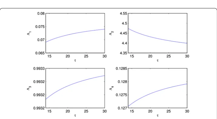
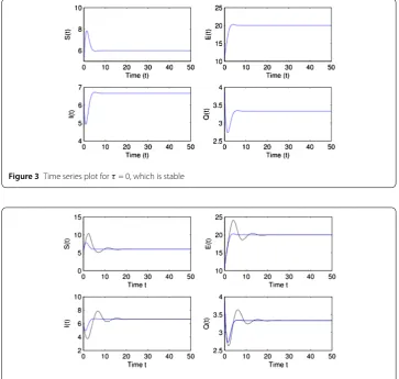
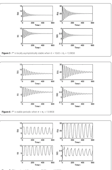
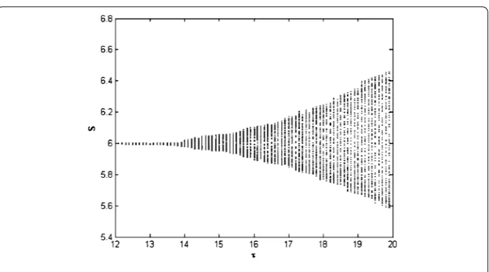
With this set of parameters we get the basic reproduction numberR0= 13.3333 > 0 and the unique endemic equilibriumP∗(6, 20.1818, 6.7273, 3.3636). Biologically it shows that all the individuals coexist. First, in the absence of latent delay, i.e.τ = 0 the dynamics of system (1) has been plotted in Fig.3and the dynamics is stable in the absence of delay (Lemma1). But in Fig.4it is seen that in the presence of delay (very small value of τ) initially all the individuals are oscillating and after some time again it comes to a stable situation. Thus for a more increased value of the delay the oscillation for the individuals also increases. Hence, the interior equilibrium pointP∗(S∗,E∗,I∗,Q∗) is seen to be stable forτ<τ0(Fig.5) and at the critical value of delay we get a stable periodic solution where the Hopf bifurcation occurs (Fig.6). Finally for large value of delayτ>τ0the system loses
Figure 3Time series plot forτ= 0, which is stable
Figure 5 P∗is locally asymptotically stable whenτ= 10.65 <τ0= 13.9858
Figure 6 P∗is stable periodic whenτ=τ0= 13.9858
Figure 7 P∗loses its stability whenτ= 28.85 >τ0= 13.9858
its stability (Fig.7). This property can be also illustrated by the bifurcation diagram with respect toτ in Fig.8.
7 Conclusions
Figure 8Bifurcation diagram with respect to time delay
some symptoms can be seen. Thus, in the incubation period it takes some time for a re-sponse to occur, i.e., delay is arising. Here, in this article we have assumed a delayed SEIQ epidemic model by incorporating the latent delay to the model proposed in [29]. Thus, compared with the model proposed in [29], the model we consider in the present paper is more general. We consider not only the effect of the time delay on the model, but also the boundedness, persistence and the properties of the Hopf bifurcation. The results obtained in the present paper are the complement of the research work in the literature [29].
For this model, a feasible regionR¯ is obtained with the appropriate choice of the pa-rameters. It can be seen that all the solutions of (2) will remain in or tend toR¯, i.e., the feasible regionR¯ is positive and invariant. If the basic reproduction numberR0> 1, then the model has an endemic equilibrium point which is unique. Also ifR0> 1 the system (2) will be persistent and forR0< 1, the infection will be extinct, i.e., system (2) becomes disease free. Next, we construct a suitable Lyapunov functional of the form (20) to check the stability of system (2). Using this Lyapunov functional the sufficient conditions for lo-cal asymptotic stability are given in Theorem1. With the choice of the parameters given in the numerical section and forτ <τ0all theare negative (Fig.1), which satisfies the conditions obtained in Theorem1. Next, the sufficient conditions for local stability of the endemic equilibrium of the model and the existence of a Hopf bifurcation are obtained by taking the delay as the bifurcating parameter. Also, the critical value of the latent delay is obtained. We can conclude that if the latent delay for system (2) is less than its criti-cal value then the endemic equilibrium for the system gets in a stable situation but if it is greater than the critical value the endemic equilibrium for system (2) will lose its stability. Further, properties of the Hopf bifurcation such as direction and stability are studied by means of the center manifold and normal form theory. At the end, with a set of suitable parameters, some numerical computations are presented to justify our results obtained analytically and to see the effect of the latent delay on the stability of the system.
τ0. In other words, the existence of these periodic solutions remains valid only in a small neighborhood of the critical valueτ0. It is interesting to investigate whether these periodic solutions remain when the value of the time delayτ becomes large enough. We leave the existence of a global Hopf bifurcation of system (2) as our next work in the near future.
= 2(μ+α+γ3) +
The authors express their gratitude to the referees for their helpful suggestions, which improved the final version of this paper. The first and the second author are thankful to the third author, for her careful guidance, without which this research would not have been possible. The second author is thankful to DST, New Delhi, India, for its financial support under INSPIRE fellowship, without which this research would not have been possible.
Funding
This work was supported by Project of Support Program for Excellent Youth Talent in Colleges and Universities of Anhui Province (No. gxyqZD2018044) and Anhui Provincial Natural Science Foundation (No. 1608085QF151), and the second author is thankful to DST, New Delhi, India, for its financial support under an INSPIRE fellowship, without which this research would not have been possible.
Availability of data and materials
All of the authors clare that all the data can be accessed in our manuscript in the numerical simulation section.
Competing interests
All the authors declare that they have no financial and non-financial competing interests.
Authors’ contributions
All authors contributed equally to the writing of this paper. All authors read and approved the final manuscript.
Author details
1School of Management Science and Engineering, Anhui University of Finance and Economics, Bengbu, China. 2Department of Mathematics, National Institute of Technology Durgapur, Durgapur, India.
Publisher’s Note
Springer Nature remains neutral with regard to jurisdictional claims in published maps and institutional affiliations.
Received: 18 May 2018 Accepted: 6 September 2018 References
1. Kermack, W.O., McKendrick, A.G.: A contribution to the mathematical theory of epidemics. Proc. R. Soc. Lond. A
115(772), 700–721 (1927)
2. Kermack, W.O., McKendrick, A.G.: A contribution to the mathematical theory of epidemics II. The problem of endemicity. Proc. R. Soc. Lond. A138(834), 55–82 (1932)
3. Billarda, L., Dayananda, P.W.A.: A multi-stage compartmental model for HIV-infected individuals: I waiting time approach. Math. Biosci.249, 92–101 (2014)
4. Pongsumpun, P., Tang, I.M.: Dynamics of a new strain of the H1N1 influenza a virus incorporating the effects of repetitive contacts. Comput. Math. Methods Med.2014, Article ID 487974 (2014)
5. Upadhyay, R.K., Kumari, N., Rao, V.S.H.: Modeling the spread of bird flu and predicting outbreak diversity. Nonlinear Anal., Real World Appl.9, 1638–1648 (2008)
7. Kermack, W.O., Mckendrick, A.G.: A contribution to the mathematical theory of epidemics. Proc. R. Soc. A115(772), 700–721 (1927)
8. Kermack, W.O., Mckendrick, A.G.: Contributions to the mathematical theory of epidemics. II, the problem of endemicity. Proc. R. Soc. A138(834), 55–83 (1932)
9. Jin, Y., Wang, W., Xiao, S.: An SIRS model with a nonlinear incidence rate. Chaos Solitons Fractals34, 1482–1497 (2007) 10. Lahrouz, A., Omari, L., Kiouach, D.: Global analysis of a deterministic and stochastic nonlinear SIRS epidemic model.
Nonlinear Anal., Model. Control16, 69–76 (2011)
11. Zhang, T.L., Liu, J.L., Teng, Z.D.: Stability of Hopf bifurcation of a delayed SIRS epidemic model with stage structure. Nonlinear Anal., Real World Appl.11, 293–306 (2010)
12. Zhang, Y.Y., Jia, J.W.: Hopf bifurcation of an epidemic model with a nonlinear birth in population and vertical transmission. Appl. Math. Comput.230, 164–173 (2014)
13. Xu, R.: Global dynamics of an SEIS epidemic model with saturation incidence and latent period. Appl. Math. Comput.
218, 7927–7938 (2012)
14. Liu, J.: Bifurcation of a delayed SEIS epidemic model with a changing delitescence and nonlinear incidence rate. Discrete Dyn. Nat. Soc.2017, Article ID 2340549 (2017)
15. Guo, S.M., Li, X.Z., Song, X.Y.: Stability of an age-structured SEIS epidemic model with infectivity in incubative period. Int. J. Biomath.3, 299–312 (2010)
16. Yang, B.: Stochastic dynamics of an SEIS epidemic model. Adv. Differ. Equ.2016, 226 (2016)
17. Witbooi, P.J.: Stability of an SEIR epidemic model with independent stochastic perturbations. Phys. A, Stat. Mech. Appl.392, 4928–4936 (2013)
18. Yang, Q., Mao, X.: Extinction and recurrence of multi-group SEIR epidemic models with stochastic perturbations. Nonlinear Anal., Real World Appl.14, 1434–1456 (2013)
19. Zhou, X., Cui, J.: Analysis of stability and bifurcation for a SEIR epidemic model with saturated recovery rate. Commun. Nonlinear Sci. Numer. Simul.16, 4438–4450 (2011)
20. Liu, L., Wang, J., Liu, X.: Global stability of an SEIR epidemic model with age-dependent latency and relapse. Nonlinear Anal., Real World Appl.24, 18–35 (2015)
21. Fan, X.L., Wang, L., Teng, Z.D.: Global dynamics for a class of discrete SEIRS epidemic models with general nonlinear incidence. Adv. Differ. Equ.2013, 123 (2016)
22. Meng, X., Chen, L., Cheng, H.: Two profitless delays for the SEIRS epidemic disease model with nonlinear incidence and pulse vaccination. Appl. Math. Comput.186, 516–529 (2007)
23. Xu, R., Ma, Z.E.: Global stability of a delayed SEIRS epidemic model with saturation. Nonlinear Dyn.61, 229–239 (2010) 24. Kuniya, T., Nakata, Y.: Permanence and extinction for a nonautonomous SEIRS epidemic model. Appl. Math. Comput.
218, 9321–9331 (2012)
25. Zhang, L.J., Li, Y.Q., Ren, Q.Q., Huo, Z.X.: Global dynamics of an SEIRS epidemic model with constant immigration and immunity. WSEAS Trans. Math.5, 630–640 (2013)
26. Gumel, A.B., Moghadas, S.M.: A qualitative study of a vaccination model with non-linear incidence. Appl. Math. Comput.143, 409–419 (2003)
27. Buonomo, B., Lacitignola, D., Leon, C.V.D.: Qualitative analysis and optimal control of an epidemic model with vaccination and treatment. Math. Comput. Simul.100, 88–102 (2014)
28. Li, J.Q., Yang, Y.L., Zhou, Y.C.: Global stability of an epidemic model with latent stage and vaccination. Nonlinear Anal., Real World Appl.12, 2163–2173 (2011)
29. Chen, X.Y., Cao, J.D., Park, J.H., Qiu, J.L.: Stability analysis and estimation of domain of attraction for the endemic equilibrium of an SEIQ epidemic model. Nonlinear Dyn.87, 975–985 (2017)
30. Li, J., Sun, G.Q., Jin, Z.: Pattern formation of an epidemic model with time delay. Physica A403, 100–109 (2014) 31. Bai, Z.G., Wu, S.L.: Traveling waves in a delayed SIR epidemic model with nonlinear incidence. Appl. Math. Comput.
263, 221–232 (2015)
32. Liu, Q., Chen, Q.M., Jiang, D.Q.: The threshold of a stochastic delayed SIR epidemic model with temporary immunity. Physica A450, 115–125 (2016)
33. Hu, Z.Y., Chang, L.L., Teng, Z.D., Chen, X.: Bifurcation analysis of a discrete SIRS epidemic model with standard incidence rate. Adv. Differ. Equ.2016, 155 (2016)
34. Li, J.H., Teng, Z.D.: Bifurcations of an SIRS model with generalized non-monotone incidence rate. Adv. Differ. Equ.
2018, 217 (2018)
35. Liu, Q.M., Sun, M.C., Li, T.: Analysis of an SIRS epidemic model with time delay on heterogeneous network. Adv. Differ. Equ.2017, 309 (2017)
36. Liu, J., Wang, K.: Dynamics of an epidemic model with delays and stage structure. Comput. Appl. Math.37, 2294–2308 (2018)
37. Sharma, N., Gupta, A.K.: Impact of time delay on the dynamics of SEIR epidemic model using cellular automata. Physica A471, 114–125 (2017)
38. Krishnapriya, P., Pitchaimani, M., Witten, T.M.: Mathematical analysis of an influenza epidemic model with discrete delay. J. Comput. Appl. Math.324, 155–172 (2017)
39. Jiang, Z.C., Ma, W.B., Wei, J.J.: Global Hopf bifurcation and permanence of a delayed SEIRS epidemic model. Math. Comput. Simul.122, 35–54 (2016)
40. Liu, J., Wang, K.: Hopf bifurcation of a delayed SIQR epidemic model with constant input and nonlinear incidence rate. Adv. Differ. Equ.2016, 309 (2016)
41. Fonda, A.: Uniformly persistent semidynamical systems. Proc. Am. Math. Soc.104, 111–116 (1988)
42. Kundu, S., Maitra, S.: Stability and delay in a three species predator–prey system. AIP Conf. Proc.1751, 020004 (2016).
https://doi.org/10.1063/1.4954857
43. Kundu, S., Maitra, S.: Dynamical behaviour of a delayed three species predator–prey model with cooperation among the prey species. Nonlinear Dyn.92, 627–643 (2018)
45. Li, X.L., Wei, J.J.: On the zeros of a fourth degree exponential polynomial with applications to a neural network model with delays. Chaos Solitons Fractals26, 519–526 (2005)