On the design of an energy harvesting noise sensing WSN mote

R E S E A R C H

Open Access

On the design of an energy-harvesting

noise-sensing WSN mote

Wilson M Tan

and Stephen A Jarvis

Abstract

Wireless sensor networks (WSNs) could potentially help in the measurement and monitoring of noise levels, an important step in mitigating and fighting noise pollution. Unfortunately, the high energy required by the noise measurement process and the reliance of sensor motes on batteries make the management of noise-sensing WSNs cumbersome. Giving motes energy harvesting (EH) capabilities could alleviate such a problem, and several EH-WSNs have already been demonstrated. Nevertheless, the high-frequency nature of the data required to measure noise places significant additional challenges to the design of EH-WSNs. In this paper, we present a design and prototype for a mote extension which enables the mote to detect noise levels while being powered by energy harvesting. The noise level detection carried out by the system relies primarily on the concept of peak detection. Results of

performance testing are presented. Aside from the hardware design and prototype, we also discuss methods of assigning charge times for application scenarios where there are multiple pulse loads. We also propose a new opportunistic method for charge time determination. Experiments demonstrate that the new method could improve analytically-derived duty cycles by at least 350%.

Keywords: Wireless sensor networks; Energy harvesting; Acoustics; Noise

Introduction

Noise pollution is becoming an increasing concern in many urban regions all over the world (for example, [1]). An important step in fighting and mitigating noise pollu-tion is its classificapollu-tion and quantificapollu-tion. Efforts being made towards this goal include cellphone applications that measure noise and noise-related legislations (such as the European Union’s Environmental Noise Directive [2] and the New York City Noise Code [3]).

Wireless sensor networks (WSNs) could potentially help with these efforts, as they could enable the simultaneous and continuous gathering of data over wide geographic regions. Several WSNs for noise pollution monitoring have been demonstrated [4-6]. WSN nodes (‘motes’) how-ever, are usually powered by batteries which have to be frequently replaced. The length of time between battery replacements depends on the energy demand of the appli-cation: for those nodes that have energy-intensive sensors, or do lots of routing, this could be days, while for nodes

*Correspondence: wilson.tan@warwick.ac.uk

1Department of Computer Science, University of Warwick, Coventry, UK 2Department of Computer Science, University of the Philippines, Quezon City, Philippines

that have simple sensors with very small duty cycles, this could be many months. The task of replacing these bat-teries on a regular basis makes the maintenance of such networks difficult.

As an alternative to batteries, WSNs could also be pow-ered through energy harvesting (EH). Several EH-WSNs have been demonstrated [7-9]; nevertheless, despite these past successes, creating an EH-WSN for noise pollution monitoring is not straightforward. The difficulty lies in the nature of the data being gathered. While a temperature-sensing WSN could probably take a reading every minute and not lose accuracy, to measure noise, sound samples have to be taken. The human ear can hear frequencies of up to 20,000 Hz - to be able to digitally reconstruct a human-audible signal without missing any frequency component, samples should then be taken at the rate of the Nyquist frequency, or around 40,000 Hz. Sampling at such a high frequency is highly energy consuming, and the processing of the data gathered is challenging to implement on resource-constrained motes.

In this paper, we present a mote extension design which would enable a mote to detect noise while being powered by energy harvesting, specifically, solar energy harvesting.

While the system doesnotconform with the standards of measure utilized by any of the existing noise codes, such a network could still be immensely useful in many urban settings - in contrast to cellphone readings taken by indi-viduals, the network could provide data and information that is uniform (since the the measuring devices would be of the same type) and properly contextualized (since each mote’s location and orientation would be known). Such data could help in building noise maps, a goal shared by many ‘smart city’ initiatives all over the world (for exam-ple, [10]). In terms of administration, our design makes for a relatively low-cost and low-maintenance system, some-thing that may not be currently achievable with WSNs that are designed to comply with existing noise codes.

A noise-sensing mote would have to regularly sample the microphone at high frequency, an operation that con-sumes a significant amount of current for an extended period of time. Using the radio for transmitting or receiv-ing messages, or even just idle listenreceiv-ing, also consumes a significant amount of energy. Such operations are called

pulse loads, as they draw pulses of high current from the energy storage device. Since both operations have to be performed in a noise-sensing mote, it can be considered to be running amultiple-pulse load application.

Energy-harvesting WSN motes usually have a boost

capacitor between itself and the energy storage device. This is to mitigate for the limits to the level of current that could be drawn from the energy storage device, imposed by the device’s internal impedance [11]. Since the capaci-tor has a finite capacity, it has to undergo repeated cycles of charging (from the battery) and discharging (to the load). This means that while a high level of current draw is now possible, such a draw could still not be sustained for an indefinite period of time - after the boost capac-itor charge is depleted, it has to be allowed to recharge or recover (in comparison, without a boost capacitor, the current draw may not be possible at all). When running pulse load applications, the charge time has to be care-fully determined to ensure that the boost capacitor is sufficiently charged before drawing any current from it. Utilizing the right charge time is of paramount impor-tance: set it too long and duty cycle (hence, performance) suffers, set it to a value too low and the system may not function at all. Fortunately, an analytical method is available for deriving the charge time of single-pulse appli-cations. Such a method however, has not been derived before for multiple-pulse load applications.

This paper presents two primary contributions: firstly, a mote extension design for noise sensing in urban environ-ments, and secondly, a discussion of charge time determi-nation methods for applications with multiple pulse loads. Aside from deriving analytical-computational methods for charge time determination, we also propose our own method, called theOpportunistic method.

The remainder of the paper is organized as follows. The next section discusses the ‘traditional’ sound level mea-surement process as carried out by WSN motes. This is followed by a discussion of our design, the rationale behind it, and the derivation of the parameter values that were utilized in it. This is followed by a discussion of power management algorithms. We then discuss the implementation of the design, how it was tested and eval-uated, and the results of the tests. In the second part of the paper, we discuss the methods available for assign-ing charge times to applications with multiple pulse loads, including our own proposed method. We then proceed to expound and describe the experiments carried out to test the effectiveness of the methods and the results of the said experiments. An overview of related and future work is then provided, after which we summarize and conclude the paper.

Sound level measurement in WSNs

Sound is a mechanical wave which uses air as a medium. As the wave travels, it induces pressure fluctuations which are then detected by the human ear, or in mechani-cal/electronic devices, a transducer. Greater energy in the wave translates to bigger pressure fluctuations, which humans then experience as theloudnessof a sound. The human ear is an extremely sensitive device: the differ-ence between the smallest and biggest pressures that the human ear can sense vary by 12-13 orders of magnitude. Representing such a huge range can be cumbersome in the linear scale, so sound pressure level (or loudness) is usu-ally defined in a logarithmic scale, with the unit ofdecibels

[12,13].

In Equation 1, Lp(t) is the instantaneous sound pres-sure level(SPL) of a sound, whilepRMS(t)is the root mean

square (RMS) of the pressure.pRMSis the standard

refer-ence pressure set at 20µPa. 20µPa is conventionally set as the minimum pressure detectable by the human ear.

pRMS(t)is not truly instantaneous since the RMS has to

be computed over a period of time. While the length of time over which the RMS must be computed is not stan-dard, it must at least be equal to or longer than the period of the lowest frequency being measured. In a discrete-time system, assuming thatp(i)is the pressure measured at the sampling instance andNis the number of samples over which we are making the RMS computation, we have

pRMS=

levels over extended periods of time isLeqT, or the time-averaged sound level. LeqT is taken from the average of

successivepRMS values. Again, assuming a discrete-time

system andN as the number ofpRMS values taken over

the time for which LeqT is being computed, we have

Equation 3 [12]:

For the microcontroller of the mote to be able to

cal-culate Equation 2, p should be in a form that is

dig-ital in nature: the pressure waveform therefore has to go through transformations. Firstly, there is the micro-phone/transducer, which senses the pressure fluctuations in the air using a thin membrane. The physical fluctua-tion of the membrane induces voltage fluctuafluctua-tions. The voltage fluctuation induced by the pressure fluctuation is defined by themicrophone sensitivity, denoted byS in Equation 4 [14]:

is the resulting voltage swing when pressure changes byp. WithSdefined (through a datasheet, for example),Ecould be easily derived from Equation 4.

The output of the microphone is a continuous voltage waveform. In most noise-measuring systems, the micro-phone output is alsoA-weighted, meaning its frequency components are attenuated or amplified to match how the human ear perceives different frequencies (since the human ear does not perceive frequencies equally [15]). The voltage waveform is also usually preamplified using an operational amplifier (op-amp)-based active amplifier before being processed by the microcontroller’s analog-to-digital converter (ADC). The ADC samples the voltage waveform in discrete time steps and discretizes the volt-age level into binary integers. The output of the ADC is a stream of binary integers, which are then stored in the microcontroller’s memory. Two parameters define the operation of the ADC: the sampling rate and the word width. A higher sampling rate translates to a more faith-ful representation of the original signal. The word width is the number of bits available for representing the sam-pled value. For instance, if the word width is only two bits, the ADC would only be able to differentiate between four levels (since 22 = 4). If the continuous voltage values vary between 0 and 1 V, values between 0 and 0.25 V would be encoded as 00 and values higher than 0.25 V but no higher than 0.5 V would be encoded as 01, etc.

The output of the ADC could already be processed by the microcontroller’s CPU and used as input to

Equation 2. While Equation 2 requires the sound pressure level, the ADC output would suffice as an input. Barring the precision loss introduced by the ADC, the relationship between the integer value and the original pressure level is linear: the output could be scaled later. Alternatively, the programmer could also choose to convert the ADC output into itsPaequivalent before having the CPU do the computation. The downsides of this approach are the extra computational steps and the need for floating point numbers, which are not supported by all microcontroller platforms.

Most noise codes rely onLeqTvalues. It must be noted

however, thatLeqTis not a perfect measure of noise,

espe-cially as experienced by people in an urban area. Since

LeqT takes the time average of noise measurement

val-ues, it is possible for intense but short noisy periods to be hidden by the measure [12]. Another important rea-son for not ignoring these short but noisy periods is the increasing amount of evidence which suggests that impul-sive noise could be more damaging than noise that is more widespread temporally [16]. As an example, take an area that is generally very quiet but regularly suffers from air-craft noise. TheLeqTmeasurement in this case would be

very low and would not reflect the disturbance caused by the aircraft passing overhead. In such a situation, thepeak

noise level detected within a time period might actually be a more informative and useful metric.

Design Design rationale

While most of the previous work that involved sound sensing has done so by recording the sound waveform [5,17,18], we have opted for an approach that is cen-tered on a peak detector, for the reasons cited above. This means that our system does not produce SPL values, but the peak noise level recorded within a period of time. Such information is insufficient for the requirements of most existing noise codes, but as discussed, such infor-mation, combined with an energy-harvesting/battery-free operation feature, would suit noise sensing in many urban settings.

Our decision to adapt a peak detector-based design is also motivated by the limited capabilities of the TelosB [19] - in a previous work [20], we demonstrated how at 10,000 Hz sampling rate, the limited memory space of the MSP430 [21,22] microcontroller only enables continuous sampling of up to 0.4 s. In comparison, for many sys-tems that monitorLeqT,pRMS is usually computed over

1-s intervals [16]. It must be noted thatLeqTcould still be

speed), but even that could be minimized by paralleliz-ing processparalleliz-ing and samplparalleliz-ing usparalleliz-ing direct memory access (DMA). Even with DMA however, two problems still remain. Firstly, the need to compute the RMS of the samples every 0.4 s would consume a lot of energy over time. Secondly, and more significantly, the number of such readings that could be accumulated would be severely constrained by the amount of space - it must be remem-bered that space is one of the factors that contributed to the 0.4-s limit in the first place. This could be allevi-ated by shorter sampling windows (i.e., shorter sampling sequences) or by frequently sending data to the sink. The former, however, would negatively affect the accuracy of the readings, while the latter would be costly in terms of energy.

In comparison, a peak detector-based system does not record the waveform at all and only generates a digital reading at the end of a sampling period. A significantly larger number of readings could then be stored, result-ing in greater flexibility in how and when such readresult-ings are processed. For example, assuming that time bounds requirements are met, readings could be accumulated so that several are sent to the base station in a single packet. The timing of sending could also be dynamically set to coincide with periods of high energy generation, helping to keep the system in energy-neutral operation. Alterna-tively, the packet sent could be externally triggered, with the data pulled out of the mote by a mobile sink or data mule. Such options are simply very limited or not available in systems that are severely constrained in the amount of data that they could store.

It must be noted that a peak detector-based design does not necessarily consume less power than a design which carries out wave sampling. The system unfortunately still has to duty cycle, meaning it cannot be in the active state all of the time. Ways of alleviating this limitation will be discussed later. While the ADC is no longer continuously active and sampling the microphone at a high frequency, a new sub-circuit is added to the system, one which con-tinuously runs during the active part of the operation cycle. Our measurements show that the power consump-tion of the sub-circuit is at par with (or just slightly smaller than that of ) an ADC at a high-frequency sampling oper-ation. Nevertheless, the flexibilities afforded by a peak detector-based system gives significantly more options for power management algorithms which could lead to energy savings in the long run.

Basic design

For our work, we used the ultra-low-power wireless sen-sor module TelosB [19]. TelosB was designed at UC Berkeley with three goals in mind: minimal power con-sumption, ease of use, and increased software and hard-ware robustness. It uses the 16-bit Texas Instruments

MSP430 microcontroller [21,22] and the 2.4 GHz IEEE 802.15.4 compliant RF transceiver Chipcon CC2420 radio [23]. The TelosB motes that we used for this work were manufactured by Advanticsys [24] and marketed as CM5000 motes. Our TelosB motes run TinyOS, or Tiny Microthreading Operating System [25,26].

For the energy-harvesting component of our setup, we utilized the CBC-EVAL-09 [27]. The CBC-EVAL-09 is an evaluation kit manufactured by Cymbet Corporation (Elk River, MN, USA). It features several energy-harvesting transducers, along with with the EnerChip EP CBC915 Energy Processor [28] and the EnerChip CBC51100 100 uAh solid state battery module (with two EnerChip CC CBC3105 [29] solid state batteries connected in parallel).

The EnerChip EP CBC915 Energy Processor [28] serves as an interface between the transducers and the energy storage device. It employs advanced maximum power point tracking tracking algorithms, constantly matching the output impedance of the energy-harvesting transduc-ers, thus ensuring high-efficiency energy conversion. The EnerChip EP CBC915 Energy Processor also facilitates communication with the microcontroller, providing infor-mation such as state-of-charge estimates and a calibration function.

For the sensor design, we utilized an ADMP401 MEMS microphone [30]. Compared to conventional electret microphones, MEMS microphones offer the advantage of minimal size, lower power usage, and a better signal-to-noise ratio (SNR) [31]. The microphone output is pream-plified by an op-amp-based inverting amplifier with a gain of 100. The preamplified output is then fed into a peak detector circuit with a load-isolated storage capac-itor. This peak detector design is more suited for long hold times than the simpler single op-amp-based alterna-tive. The details of the peak detector design are discussed in detail in [32-34]. The output of the peak detector is connected to ADC channel 0 of the TelosB, where it is sampled at the end of a sensing period. All three oper-ational amplifiers (op-amps) utilized in the design are OPA344s [35].

To facilitate duty cycling, the supply lines of the micro-phone, the preamplifier, and the peak detector are gated by the high-side switch ADP194 [36]. The ADP194 is dig-itally controlled by the TelosB using a digital I/O pin. During the sensing period, theEnablepin of the ADP194

is set to high by the TelosB, enabling the current to

flow to the microphone, the preamplifier, and the peak detector.

causes it to have an overshot output in the beginning of a sampling period. To return the output to its normal level, a ‘corrective discharge’ is carried out by con-necting the capacitor to the discharge resistor for a few milliseconds. Like the ADP194, the MAX323 is digitally controlled by the TelosB using a digital I/O pin.

The schematic of the expansion board (which contains the microphone, preamplifier, and peak detector) is shown in Figure 1.

Design parameters - sensing side

The first design parameter that needed to be derived was the value of CCh, or the storage capacitor. The storage

capacitor stores the voltage that corresponds to the max-imum loudness of sound that has been observed within an active period. It is connected directly to the ADC port of the microcontroller, which samples the voltage level of

CChat the end of an active period. TheCChis discharged

after sampling so that it could start at a very low level in the next active period. It must be noted that the stor-age capacitor is different from theboost capacitor, the value of which would also be derived in a later subsection. The size of the storage capacitor depends on the charging speed required of the system, which in turn depends on the desired sound frequency range covered by the detec-tor. The maximum rate at which the the voltage acrossCCh

could change is either

dVCh

dt =SR1 (5)

or

dVCh dt =

IOmax CCh

, (6)

whichever is smaller [32]. The values of SR1and IOmax,

or the slew rate and short-circuit current ofOP-AMP 2in Figure 1, are specified by the datasheet [35] as 0.8V_µs and 15 mA, respectively. TheCCh is then dependent on the

desired rate of voltage change. To derive this, we assume a maximum sound frequency of 10,000 Hz and require the system to be able to swing from the quiescent level to the upper rail (a 1.5 V swing) within a single cycle. A maximum frequency of 10,000 Hz was chosen for the ini-tial design because most of the frequencies to which the human ear is sensitive can be found below 10,000 Hz [15]. Referring to Figure 2, assuming thatVSwing ≈ VAmplitude

andt1≈t2, we can simplify the computation ofdV_dtCh as

dVCh dt =

VSwing

2×t1

(7)

Remembering thatt1is 1 10000

4 , Equation 7 gives 30,000Vs ,

which is smaller than SR1. This means that the speed is

supportable by the operational amplifier subject to the correctCChvalue. Substituting this value into Equation 6

and solving forCChgives us 0.5µF.

Ideally, the output of the peak detector should remain stable until a higher peak than the previous is seen in the input. In reality, the peak detector output decays over time due to leakage current (an effect calledvoltage droop[32]). The rate of discharge ofCChis

Figure 2Diagram demonstrating simplifying assumptions adopted for parameter computation of_CChsize.

Voltage droop= Ilk

CCh

, (8)

whereIlk is the leakage current. There are five sources of

leakage current, namely: capacitor leakage, printed circuit board leakage, op-amp leakage, diode leakage, and reset switch leakage.

With the exception of op-amp leakage and diode leak-age, all components ofIlk are difficult to quantify. Diode

leakage is negligible since an ultra-low-leakage diode was utilized for the design. That leaves the op-amp leakage or the input bias current of the op-amp, which the datasheet

gives as 10 pA maximum. Thus, Ilk = 10 pA. Using

Equation 7 and the value derived forCCh, this gives us a

voltage droop of 0.00002V_s .

The voltage droop simply gives the rate at which the output of the peak detector decays over time. The actual decrease in the output depends on how much time has elapsed since the peak value was stored by the circuit. Since we do not know the exact time at which the peak detector stored a new peak value, this introduces uncer-tainty in the output. This output is further affected by the length of the active period (which is dictated by the duty cycle, to be discussed later). Since the microcon-troller does not sample the peak detector output until the end of an active period, the longer the active period, the more opportunity there is for the inaccuracy of the peak detector output value to increase - this is especially true for peak values that are recorded very early on in the active period.

Design parameters - power supply side

The amount of current that could be drawn from an energy storage device is limited by the device’s internal

impedance. To compensate for this, a capacitor is usu-ally inserted between the energy storage device and the load. This capacitor would be called theboost capacitor, to differentiate it from thestorage capacitorwhose size was derived in a previous subsection. For the sake of brevity however, all references to ‘capacitor’ should be taken to mean ‘boost capacitor’. It must be noted that since the electrical charge has to be transferred from the energy storage device to the capacitor, it is still impossible to sup-ply a high amount of current to the load for indefinite periods of time.

For the same level of current draw, a longer draw period would necessitate using a larger capacitor to store a greater amount of electrical charge from the primary energy storage device. However, a larger capacitor also takes longer to charge - therefore, the intervals between

current draws, which we also callcharge time, would also increase.

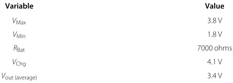
The relationship between the capacitor size, the level of current draw (in milliamperes), the length of the current draw, and the interval between draws could be derived analytically and computed: for instance, the energy stor-age system that we utilize for our work, the EnerChip CC CBC3105 [29], specifies through an application note [11] a formula for determining the capacitor size needed for supporting a specified level of current draw for a specified length of time. We state this in Equation 9. The equation for RLoad, which is a variable in Equation 9, is defined

in Equation 10. Equation 9 and Equation 10’s variables are defined in Table 1. For variables whose values remain constant across different computations, their values are specified in Table 2.

C= tDraw RLoad×ln

VMax VMin

(9)

RLoad =

Vout (average) Ipulse

(10)

The formula for the charge time of a given specific capacitor is also given by [11], and is stated here in Equation 11. Equation 11’s variables are also defined in Table 1.

tCharge = −RBat×C×ln

VMax−VChg VMin−VChg

(11)

Solving Equation 9 and Equation 11, for example, a system utilizing a 5,000 µF capacitor should be able to support a current draw of 20 mA for 210 ms with a charge time of 45 s.

Defining duty cycle as the proportion of time the system is awake or active in a cycle, we now have Equation 12

dutycycle= tDraw

tDraw+tCharge

Table 1 Equation 9 - Equation 12 variables

Variable Description

C Capacitance of external capacitor in parallel with the battery

tDraw Length of time that the current would be drawn

RLoad Load resistance

VMax Final capacitor voltage that must be attained before next current draw

VMin Initial voltage when charging begins

tCharge Capacitor charge time

RBat Battery resistance

VChg Applied charging voltage on the capacitor

Vout (average) Average voltage across the load during the current draw

Ipulse Level of current draw(inAmperes)

Substituting Equation 9 and Equation 11:

dutycycle= RLoad×ln

VMax VMin

RLoad×lnV_VMax_Min −RBat×lnV_VMax_Min−−_VV_ChgChg

(13)

It must be noted that the only variable defined by the load which appears in Equation 13 isRLoad. Referring to

Equation 10, onlyIpulse determines the duty cycle of the

system. The capacitor, in particular, does not figure in Equation 12. A larger capacitor would enable a longer draw time, but its ratio to the sum of the charge time and the draw time (thetotalperiod) would always be the same. In some applications, the length of the current draw may be user-definable. An example of such a load would be the microphone. To have a longer draw time, we may opt for a larger capacitor, but the interval between draws would proportionately increase as well. In other applications, the length of the current draw is already defined. An exam-ple of such a load is a radio which has to send a message to a receiver which is duty cycling using low-power listen-ing (LPL) [38]. If the wake-up interval of the receiver has already been decided or set, the designer has no choice on the size of the capacitor that must be installed on the sender.

Traditionally, duty cycling was seen as a necessity imposed by the limited amount of harvested energy. As

Table 2 Equation 9 to Equation 12 variables and values

Variable Value

VMax 3.8 V

VMin 1.8 V

RBat 7000 ohms

VChg 4.1 V

Vout (average) 3.4 V

can be seen in Equation 13 however, the hardware imposes its own cap on the duty cycle feasible. It is interesting to note that neither the storage size nor the solar panel output figures in Equation 13. Therefore, using larger bat-teries or larger solar panels will not help in solving the limit imposed by Equation 13.

If higher duty cycles than that imposed by Equation 13 are desired or needed, a possible solution would be to co-locate several sensor nodes. Enough nodes should be co-located so that the temporal coverage required is sat-isfied. If, for example, Equation 13 imposes a limit of 25% and 100% duty cycle is required, four nodes should be co-located, with the nodes taking turns in being active. The primary challenge in this solution would be the tight synchronization that would be required of the co-located nodes, and its main disadvantage would be the cost. A schematic for node co-location is shown in Figure 3.

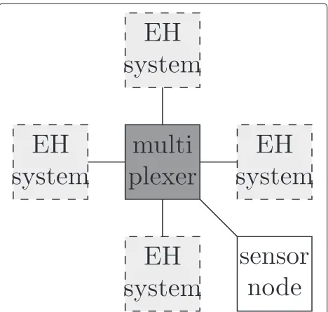
Another possible solution would be to use one node with several energy-harvesting systems, each with its own solar panel and energy storage device. Upon depletion, the node would simply switch energy-harvesting systems, allowing the previously used system to recharge. As with the previous example, if there is a 25% limit, but a 100% duty cycle is required, four energy-harvesting systems would now be required. This would be less costly than the previous solution, and no synchronization would be needed, but there is the challenge of ensuring that the multiplexed power supply would be able to provide a supply level that is stable enough for continuous system operation. To the best of our knowledge, switched or mul-tiplexed power supplies have never been used before in the context of overcoming duty cycle limitations in WSN nodes. The closest previous work is [39], where differ-ent subsystems in an embedded system were allowed to be powered simultaneously by different energy sources in an attempt to maximize energy harvesting efficiency. The schematic for node co-location is shown in Figure 4.

sensor

node

EH

system

sensor

node

EH

system

sensor

node

EH

system

sensor

node

EH

system

Figure 4Power supply multiplexing schematic.

It must be noted that node co-location and power supply multiplexing only change the upper limit imposed by the physical system with regard to the maximum duty cycle achievable. Theactualachieved duty cycle is still a func-tion of the harvested energy and the energy usage pattern of the application. The amount of harvested (and stored) energy is affected by the node’s location, harvesting effi-ciency, solar panel size, and storage capacity. The energy usage pattern of an application is usually tailored to the energy state of the system and the environment by power management algorithms. Power management algorithms are discussed next.

The microphone, preamplifier, and peak detector por-tion of our circuit was measured to have a collective current draw of 0.8 mA, translating to a duty cycle of 9.9%. We chose the boost capacitor size of 11,000µF for a draw time of 10.05 s and charge time of 91.0 s. We believe that such values give an acceptable trade-off between the length of the draw time and the interval between the draws.

Power management

For an actual deployment to function, the motes need a power management algorithm. The power management algorithm manages the power consumption of the system, ensuring that system operation stays stable and functional despite variations in harvested energy. An obvious task for the power management algorithm would be adapting the system operation to the diurnal cycle, making sure that enough energy is harvested during the day so that the sys-tem remains functional even at night. The choice of power management algorithm would depend on several factors:

the application type, the network topology, and the hard-ware available. We do not include a specific algorithm since the mote could be used for different types of appli-cations and different network topologies. We do, however, discuss the factors that guide the choice and design of an appropriate power management algorithm.

Application type

Strictly speaking, a power management algorithm is any algorithm which changes an aspect of the system to meet energy constraints. What aspect is actually changed could vary from one algorithm to the next. For systems that reg-ularly sample a single sensor, what is usually varied is the duty cycle. In [40], for example, the algorithm takes into account the predicted energy that would be harvested and assigns duty cycles to time periods calledframes. The duty cycle assignment ensures that the node only consumes what it harvests, resulting in an infinite lifetime, or a mode of operation calledenergy-neutral operation. It also makes provision for when the actual harvested energy deviates from that which was predicted, increasing the duty cycles in subsequent frames when more energy is harvested than predicted and reducing the duty cycles when less energy is harvested. A power management algorithm such as that featured in [40] would be a possible good fit for systems that utilize our mote, although modifications are neces-sary. For example, [40] assumes that there is a utility level associated with the duty cycle and that there is a maxi-mum duty cycle beyond which the utility would no longer increase. Even without an explicit consideration of util-ity however, in our system, the hardware already explicitly imposes a limit to the duty cycle. Such a limit would have to be taken into account when using the algorithm in [40]. Other power management algorithms (such as [41]) assume that the processor or microcontroller is capable of dynamic voltage and frequency scaling (DVFS) and thus changes the speed of the processor or microcontroller in accordance with the energy state of the system. This is not applicable to our system since the microcontroller of the TelosB, like other low-power microcontrollers, does not have the DVFS feature.

A mote could also possibly change the sensor or set of sensors being used in response to the energy state [42]. This is more applicable to motes that use multiple sen-sors, which is currently not the case in our prototype (although it could be easily extended with other sensors; for instance, one could simply activate one or more of the onboard sensors of the TelosB).

Other algorithms facilitate power management by controlling the sequence or start time of tasks [44]. Algorithms that belong to this family are more suited for embedded systems that react to real-time events, rather than those designed for regular data gathering.

Network topology and configuration

The network topology and configuration also have an effect on the power management algorithm as it deter-mines the additional tasks that a node has to do, in addi-tion to sensing and sending its own data. The tasks change the characteristics of the application (for example, its peri-odicity) and the power management techniques that are applicable.

Topology-wise, networks could be divided into two: single-hop networks and multi-hop networks.

Nodes in multi-hop networks (except leaf nodes) have the additional task of acting as a relay for other nodes -therefore, they do not just send messages, but receive messages as well. How much energy is spent on this task depends largely on the number of other nodes the node is serving as a relay for, and the media access control (MAC) protocol utilized. The nodes could communicate either synchronously or asynchronously. In synchronous com-munication, message transmission consumes relatively little energy, but there is the challenge of regular clock synchronization (which consumes energy itself ). Such an approach is utilized in [45]. Asynchronous communica-tion like LPL does not need synchronizacommunica-tion but could potentially consume more energy than synchronous com-munication (in LPL, the energy is usually spent by the sender, mainly in sending the prolonged preamble) and could possibly suffer from congestion.

Nodes in single-hop networks do not have to relay mes-sages for other nodes, but depending on the terrain and deployment environment, such a topology may not always be feasible. Single-hop networks could be push-based, where nodes regularly send their data to a sink, or pull-based, where the nodes only send data after receiving a request to do so. The latter is usually used in systems where the base station is mobile and travels around the deployment area collecting accumulated data from the nodes.

Hardware

The hardware available for energy measurement/estima-tion affects the choice of power management algorithm. All power management algorithms assume the availabil-ity of some sort of information about the energy state of the system or the environment, and the availabil-ity and accuracy of that information depends on the hardware.

Kansal et al. [40] for instance, assume that the amount of energy being harvested is always known, a reasonable requirement given that the Heliomote [46], for which the

algorithm in [40] was designed, is equipped with ded-icated circuitry that measures the voltage and current (hence, power and energy) coming from the solar pan-els. Without dedicated hardware, motes could measure the energy state of the system by measuring the voltage level of the energy buffer (usually a rechargeable battery or capacitor). It must be noted however that the battery voltage indicates the combined effect of the energy har-vesting and the energy consumption. Unless all loads are turned off, the actual amount of energy being harvested cannot be known. Even if the loads could be turned off, the buffer voltage level usually rises very slowly in response to changes in energy level and could therefore only offer energy data of poor resolution.

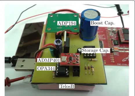
Physical setup and testing

An expansion board for the TelosB was created incorporat-ing the sensor and other circuit extensions (see Figure 5).

Basic system operation, as seen through the output of the peak detector (sensor) and the microphone, is plotted in Figure 6. In the graph, the sampling period started at 57.8 s and ended at 69 s. The overshoot in the peak detec-tor output at the beginning of the sampling period can be clearly seen, as well as its correction, brought about by the corrective discharge. Sound, generated through human speech, is generated at 60.0 s. The sound lasted for almost a second, and the peak detector output can be seen ris-ing to the peak level of the sound. The retainment of the peak detector of the sound’s peak level can be seen, even after the cessation of sound generation. It must also be noted that the voltage droop exhibited by the system is larger than that computed in a previous section, suggest-ing that the leakage current, orIlk, was underestimated in

the computations.

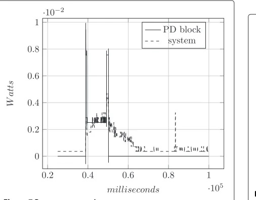
The power consumption of the system (and the peak detector block alone), as it goes through the different

Figure 6Sample operation.(A) beginning of active period. (B) Corrective discharge. (C) Sound is introduced. (D) Cessation of sound. (E) Sampling and discharging of storage capacitor. (F) End of active period.

phases of operation, is plotted in Figure 7. It can be seen that even when the peak detector block (which includes the MAX323 and the microphone) is not active, the sys-tem has a quiescent power consumption of 0.36 mW. When the peak detector block is active, power consump-tion rises, with a peak of 2.8 mW.

To test the system, the board was exposed to three dif-ferent kinds of sound, of differing loudness levels. The three different kinds of sound utilized were 10,000 Hz tone, white noise, and pink noise. White noise is a random signal with flat or constant power spectral density, and pink noise, on the other hand, has a power density which is inversely proportional to the frequency. The sound was produced in 1-s pulses fired in succession with

inter-Figure 7Power consumption.

pulse gaps of random lengths. The possible inter-pulse gap lengths however, were limited in such a way that at least a single pulse would be fired within any active period of the system. This is so that ‘soundless’ active periods would not skew the average of the readings. Random gap lengths were used so that we could test the effects of dif-fering sound introduction points in an active period. The sound level was verified by a sound level meter (SLM) located very near to the mote’s microphone. In between each active period, a packet is sent to the base station: the packet contains the reading made in the preceding active period. The mote was powered via energy har-vesting in all of the experiments, with the solar panel illuminated by a lamp shining with a brightness of at least 1,300 lx. Before any of the experiments, the solar panel and the EH system were exposed to the light for 50+ min without any load to ensure that the batteries are fully charged once the experiment begins. Each experiment lasted for a duration which enabled the system to take 20 readings.

The values produced by the system in the experiments are plotted in Figures 8, 9 and 10. It must be noted that Figure 8 has no data for 110 dB because of the limits imposed by our audio equipment. Figures 8, 9 and 10 show that the system could differentiate between differ-ent sound levels. The graphs are sigmoid in shape, with the tapering in higher decibel values indicating the micro-phone’s limitation in differentiating very loud sounds (those greater than 100 dB). Likewise, the baseline value and the first bars on the left-hand side show that the microphone could not detect sound level intensities lower than 50-60 dB.

Using the data from the white noise experiment and exponential regression, we were able to find a function relating the sensor output to dB level. We removed the last data point (110 dB) since the resulting function no

Figure 9White noise test.BL, baseline (no sound generated), all other numbers in the X-axis have dB as units.

longer tracked the data points well. The resulting function is shown in Equation 14:

f(x)=0.518203434173811×1.00708470990609x (14)

The function, along with the experimentally-derived data points, is plotted in Figure 11. Below 70 dB, the func-tion’s maximum deviation from the actual value goes up to 7 dB. Beyond 70 dB, the maximum deviation goes down to 4 dB.

Theoretically, a table of finer resolution could be pro-duced, which would enable a more accurate discernment of sound levels.

Methods for computing charge time in multiple-pulse load applications

For systems with only a single pulse component or only one component/function which consumes a large amount of current for an extended period of time, Equation 9

Figure 10Pink noise test.BL, baseline (no sound generated), all other numbers in the X-axis have dB as units.

Figure 11Function derived from curve-fitting the data points generated through experimentation.f₍x₎₌0.518203434173811_× 1.00708470990609x_.

and Equation 10 would suffice in deriving the size of the capacitor needed. Equation 13 would then give the duty cycle of the system. For applications that have two or more components that have significant current draws (or what we callmultiple-pulse load applications), however, Equation 9 and Equation 10 would not suffice.

should be the size of the boost capacitor, and what should the intervals (charge times) be between the pulse loads?

In this section, we consider the case wherein there are two pulse loads in the system. Nevertheless, all of the methods could be easily and readily extended to accom-modate three or more pulse loads.

References would be made tosmallerandlarger pulse loads. By this we mean with respect to the size of the boost capacitors computed for each pulse load using the method described earlier in the paper.Pulse loadswill also be referred to simply asloads. Once again, since all capac-itors involved in this subsection are boost capaccapac-itors, all references to ‘capacitors’ should be taken to mean ‘boost capacitors’.

For all the methods described, the capacitor of the larger load is utilized (which easily answers the first part of the problem posed above). The larger capacitor is uti-lized because it will accommodate both current draws. The capacitor of the smaller draw could possibly prove insufficient for the larger draw, completely depleting it or dropping its voltage below the minimum level required for system operation.

Lazy method

In the simplest of the four methods, the computationally-derived charge time for the larger of the two loads (the one needing a larger capacitor) is simply used for both loads. The method is guaranteed to work: since the charge time is enough to recharge the capacitor after a large current draw, it would definitely suffice for the smaller current draw. The main advantage of the method is its simplicity, while its main disadvantage is the performance loss that comes with it. The charge time of the larger draw is usu-ally larger than that of the smaller draw’s original charge time - thus, the overall duty cycle of the system would be lower than what it would be if the two draws were simply concatenated. Since the smaller draw does not deplete the capacitor as much as the larger draw, it follows that the smaller draw could actually make do with a shorter charge time - something which would be taken advantage of by another method.

Concatenation method

In this method, the two or more loads are simply concate-nated, or executed in sequence, each retaining its original, analytically-derived charge time. The reason this method can work is primarily because of the inherent conserva-tiveness of the analytical method, and indeed, preliminary experiments have shown that this method can work for certain combinations of loads. The main advantage of this method is its simplicity: the computations necessary are exactly the same as that of the single-load system, only performed several more times. The disadvantage of this method is that it does not work for all load combinations:

when the loads are vastly different in magnitude, the capacitor may not have enough time to be charged at a sufficiently high enough voltage level before the next load manifests itself.

Aggressive analytical method

In this method, the analytical method is optimized to reflect the fact that while there are now two different loads in the system, there is only one capacitor. The value of the heavy load charge time would remain the same -although it would now become the charge timeafterthe execution of the heavy load andbeforethe execution of the light load. This is because the capacitor’s recovery time after a heavy load should remain the same as before - it is the heavy load’s optimal capacitor size that is being used in the system after all. What will change and be newly com-puted by this method is the charge timeafterthe light load andbeforethe heavy load. To compute this:

1. Denote thetDrawandRLoadof thelight load as tDrawLightandRLoadLight, respectively, and denote the

optimal capacitor size for the heavy load asC, computeVMinLightwith

VMinLight=

VMax

e

t_DrawLight RLoadLight×C

(15)

This is, in effect, the level at which the voltage across the capacitor will drop to when the light load makes its current draw.

2. ThetChargefor the light load (denoted astChargeLight)

could then be computed from Equation 2, using

VMinLightinstead ofVMin.

Opportunistic method

analytical method, the value that must be assumed is the minimum supply rate, or at most, the average. Thus, there are moments wherein the system could actually support better performance (i.e., higher duty cycles). When pre-dictability and regularity are not strictly required, such extra performance not being utilized could be considered aswastedperformance.

To avoid such waste whenever possible, we propose a new method for charge time determination. Instead of utilizing predetermined charge times for a load, an

opportunisticcharge time is instead used: the system will execute a load whenever possible, subject to the charge level of the capacitor. For this, we rely on the MSP430’s supply voltage supervisor (SVS), which also has counter-parts in other microcontrollers. The SVS, when activated, continuously monitors the level of the supply voltage of the microcontroller, and sets theSVSOPbit of the 8-bit

SVSCTL register to 1 whenever it goes below a user-predefined value. The enabling and disabling of the SVS, as well as the setting of the voltage threshold, are like-wise done by setting certain bits in theSVSCTLregister. To implement the method, the execution of the load must be gated or wrapped by another code which activates the SVS and checks theSVSCTLregister. The pseudocode for such wrapping or gating, calledGated_Exec, is outlined in Algorithm 1.

Algorithm 1 Wrapping/gating code for Opportunistic Algorithm

1: procedureGATED_EXEC(volt_limit,thresh_count) 2: threshold_exceeded=False

3: threshold_exceeded_counter=0 4: low_power_flag=0

5: whilethreshold_exceeded_counter<thresh_countdo

6: Delay (1s)

7: Enable SVS Monitoring, define low voltage as

volt_limit

8: Delay (10ms) Allow SVS monitor to settle

9: From SVS register, setlow_power_flagvalue

10: Disable SVS Monitoring

11: iflow_power_flag=1then

12: threshold_exceeded=False

13: else

14: threshold_exceeded=True

15: end if

16: ifthreshold_exceededisTruethen

17: threshold_exceeded_counter=

threshold_exceeded_counter+1

18: threshold_exceeded=False

19: else

20: threshold_exceeded_counter=0

21: end if

22: end while

23: Execute Load

24: end procedure

The code is parameterized by two values:volt_limitand

thresh_count. Lines 5-22 comprise the main while loop of the code which prevents the execution of the load while conditions are not yet met, primary of which is the

threshold_exceeded_counterreachingthresh_count. Line 6 imposes a 1-s delay between loop iterations. Line 7 enables the SVS and sets the voltage threshold (defined by the user throughvolt_limit). Line 8 gives time for the SVS to set-tle. In Line 9, theSVSOP bit of the SVSCTLregister is checked, and its value copied tolow_power_flag. Line 10 disables the SVS between loop iterations, to save power. Lines 11-15 check the value of thelow_power_flag, effec-tively converting it to a boolean variablethresh_exceeded. A value of True for thresh_exceeded indicates that the supply voltage has exceeded that of the threshold. Lines

16-21 deal with determining the new value of

thresh-old_exceeded_counter: it is incremented by 1 if the thresh-old is exceeded (thresh_exceeded isTrue) and reset to 0 otherwise. The purpose of the parameterthresh_count(to whichthresh_exceeded_counter is compared) is to allow users to define a minimum amount of time by which the threshold voltage level must be exceededcontinuously

before considering the capacitor as sufficiently charged for load execution. This is important since the relationship between capacitor voltage and its state of charge is not linear - the rise of capacitor voltage slows down during the latter stages of the charging process. Thus, even if the threshold is set to a high value, it would not be pru-dent to immediately consider the capacitor as sufficiently charged just because its voltage was observed to surpass the said threshold - this is especially true for capacitors of significant size. Another use for this parameter is for rate control in routing protocols such as directed diffu-sion [48]. In directed diffudiffu-sion, a node on the path to the sink may request upstream nodes to slow the generation of data or packets because it could no longer handle the packet volume. The execution of the actual load happens in Line 23, which will only be reached upon escaping the loop embodied in Lines 5-22.

Testing the methods for computing charge time in multiple-pulse load applications

sender would stop the send upon receiving an acknowl-edgement from the receiver, to save energy. The capacitor sizes and charge times for the four loads (Load 1, Load 2A, Load 2B, and Load 2C) when each is considered in isola-tion are tabulated in Table 3.

To test that the setups are working, all the packets are received by the base station, which indicates packet recep-tion through a terminal printout. The system was powered by energy harvesting during the experiments, with the same conditions as that in the previous experiment (same light intensity, pre-experiment exposure). In each setup, the capacitor utilized was that of the larger load: for exam-ple, in the Load 1-Load 2A setup, the capacitor used was 5,000 µF. Each experiment ran for a period sufficient enough so that 25 packets from each type of send was sent by the mote.

All methods were tested on all three setups and found to be functional. For the Opportunistic method,

thresh_countwas set to 1, andvolt_limitwas set to 3.35 V, for both loads. The application running on the mote was slightly modified for the experiment used to test the Opportunistic method - to enable us to keep track of the charge times, the length of the charge time preceding a send was sent within the packet as payload. The length of the charge time can be determined by the number of iter-ations of the loop embodied in Lines 5-22 of Algorithm 1. To ensure that the system is in continuous operation (not restarting), each packet also contained a sequence number that was regularly incremented after a send operation.

For the Load 1-Load 2B setup, Figure 12 plots the oppor-tunistically determined charge times for both loads, along with the charge times determined by the Concatenation method.

It can be seen in Figure 12 that the opportunistically-derived charge times vary across time, indicative of the constantly changing charge rate of the energy-harvesting system. It must be noted that in the opportunistically-derived pair, the charge time for the heavy load is always smaller than that of the light load, in contrast with the analytically-derived pair. To understand this, one must remember our definition of charge time: it is the period of time before a current draw (or active period). A light load is preceded by the heavy load, which draws a signif-icant amount of current from the capacitor. Thus, charg-ing the capacitor to an acceptable voltage level would

Table 3 Load table

Draw length (s) Capacitor size (uF) Charge time (s)

Load 1 0.26 2,000 29.18

Load 2A 0.63 5,000 70.7

Load 2B 1.02 8,000 114.5

Load 2C 1.42 11,000 157

0 5 10 15 20

0 20 40 60 80 100 120

packet sequence number

charge

time

(seconds)

Light Load Opport. Heavy Load Opport. Heavy Load Concat. Light Load Concat.

Figure 12Charge times: Opportunistic method vs Concatenation method.

take time. By the same token, the heavy load is pre-ceded by the light load, which relatively does not draw much current. Therefore, it may be more prudent to compare the opportunistically-derived heavy load charge time with the analytically-derived light load charge time, and vice versa. Even when such comparisons are made however, the opportunistically-derived values are still sig-nificantly less than that of the analytically-derived values. For instance, the average opportunistically-derived charge time for the light load is 19.25 s, and the analytically-derived charge time for the heavy load is 114.5 s.

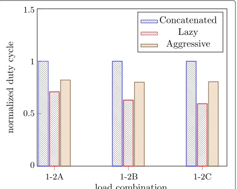
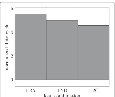
The duty cycles associated with each method for the three setups are normalized against that of the Concate-nation method and plotted in Figure 13 and Figure 14. Figure 13 plots the duty cycles associated with the three

Figure 14Normalized duty cycles, Opportunistic method.

analytical methods, while Figure 14 plots the average duty cycle measured when the Opportunistic method is used. The data for the Opportunistic method was plotted sep-arately since its numbers are significantly larger than that of the other three.

Figure 13 shows the Lazy method and the Aggressive Analytical method being inferior to the Concatenation method. This is to be expected. As already mentioned, the Lazy method is guaranteed to work but has the drawback of performance loss, which grows proportionately with the disparity between the sizes of the light load and the heavy load. This too, is apparent when the results are com-pared across setups. The Aggressive Analytical method performed better than the Lazy method, but still worse than the Concatenation method. The Aggressive Analyti-cal method is also guaranteed to work, but even with the other charge time tailor-fitted for the voltage drop caused by the light load, the value is still larger than that of its counterpart in the Concatenation method. The voltage level from which the charge period has to recover is higher (because the capacitor is larger), but the capacitor is now also more difficult to charge.

Figure 14 shows normalized data for the Opportunistic method. The Opportunistic method performed signifi-cantly better than all three other methods, with the lowest in the three setups showing a 350% improvement over the Concatenation method. These results signify that if the requirements of perfect data regularity and predictability could be relaxed, significantly more performance could be had from the system.

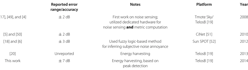
Related work

Noise measurement using WSNs has been attempted four times before: firstly, in the work presented in [17], [49],

and [4]; secondly, in the work presented in [5] and [50]; thirdly, the work presented in [18] and [6], and most recently, our own work in [20].

Compared to the research presented in this paper, the first and second sets of studies are more complete end-to-end solutions for noise monitoring: they employed A-weighting and have customized networking protocols (presented in [49,50], respectively). The third study is notable for its use of fuzzy logic in inferring subjec-tive noise annoyance from the sensor readings. Tan and Jarvis, 2013 [20], on the other hand, featured the first noise-sensing WSN motes to be powered by energy harvesting.

Table 4 summarizes the main differences between these previous studies.

This work is, in a sense, a direct follow-up to [20]. Tan and Jarvis, 2013 [20] discussed the difficulties of noise sensing using low-power WSN motes, difficulties that are compounded further by having the motes pow-ered by energy harvesting. These difficulties include the limited storage space available for the microphone volt-age readings, and the limited word width of the system. Both place limits on the length of time over whichLeqT

could be taken. This work, in comparison, does away with

LeqTand uses the peak noise level detected within a time

period instead. This design decision, brought about in part through discussions with domain experts at New York’s Center of Urban Science and Progress (CUSP), leads to the minimization of the need for high-frequency ADC sampling, making limited storage space and word widths much less of an issue. Therefore, the continuous and uninterrupted period of time over which the mote could make its observation is much longer than in [20]. While no noise codes currently employ peak noise levels as their metric, it is still very deployable in many situations and would complement other noise-sensing systems that

employ LeqT as a measure. Moreover, our design being

powered by energy harvesting makes it a good fit for low-maintenance urban sensing systems.

Table 4 Comparison of previous studies

Reported error Notes Platform Year

range/accuracy

[17], [49], and [4] ±2 dB First work on noise sensing; Tmote Sky/ 2008

utilized dedicated hardware for TelosB [19] noise sensingandmetric computation

[5] and [50] _±2 dB CiNet [51] 2010

[18] and [6] ±3 dB Used fuzzy logic-based method Sun SPOT [52] 2012

for inferring subjective noise annoyance

[20] Unreported Energy harvesting TelosB [19] 2013

This work ±7 dB Energy harvesting, based on TelosB [19] 2014

peak detection

Even without the detailed technical study however, one aspect of the competing systems could already be com-pared: cost. The Waspmote is a ready-for-deployment system. The cost of the Waspmote and Smart Cities sensor board combination (sansenergy-harvesting com-ponent) is 270 Euros. In comparison, the TelosB is a prototype/research platform costing 77 Euros. The energy harvesting system that we have utilized is part of an eval-uation board package, but a cursory check of individual component costs indicate that the total cost of compo-nents for the energy-harvesting system does not exceed 30 Euros. The cost of the customized sensor board comes in at under 20 Euros. All in all, the cost of a fully customized TelosB-based system (in a single board) is less than half the cost of an equivalent Waspmote-based system, even if only a modest number of units are produced.

Future work

Planned future work for our mote extension design includes trying out new microphones to extend the range of sound intensities which the system could discern. In due course, we also intend to incorporate A-weighting to our design, either via a software implementation or a separate circuit.

Of primary concern in future design iterations is the voltage droop, which computations underestimated for the current design. Two strategies could be adopted: com-pensation and reduction.

We can opt to compensate for the voltage droop by adjusting the digital sampling strategy. In this work, a dig-ital sample is taken at the end of the peak detector’s active period. To compensate for the voltage droop, we could take several digital readings within an active period and just keep the highest among them. The main disadvan-tage that comes with this approach is the increased storage space utilization and operational complexity.

We can also aim for the outright reduction of voltage droop. This could be done by a better circuit board lay-out, or by using better op-amps. The storage capacitor size could also be increased (Equation 8), but in doing so, the

range of frequencies detectable by the system would then decrease (Equation 6).

In this work, we also optimized the charge time of a cycle by monitoring the voltage of the boost capacitor (which is indicative of the capacitor’s charge level) instead of relying on a precomputed value. A cycle has two parts: the active part (the current draw time) and the inactive part (the charge time), and our work optimized the lat-ter. In the same way that the analytical method is very conservative in its charge time computation, and it is also very conservative in its capacitor size computation. Our experiments showed that the capacitor computed for a certain length and level of current draw could actually support a much longer current draw than what it was orig-inally intended for. We presented methods for deriving the actual maximum current draw length that a capaci-tor could support in two previous studies [54,55]. While the value could be derived manually via experimentation, what is unique about the techniques presented in [54,55] is that they allow the nodes to derive the values themselves, without human intervention, even while in deployment. This allows nodes to tailor and optimize their operations in response to conditions that affect the capacitor, such as capacitor ageing. While the techniques presented in [54,55] were done in the context of a very specific type of pulse load (radio communication using LPL), gener-alizing the techniques is certainly possible. Part of our future work then is combining the work done in this paper with generalized versions of the techniques presented in [54,55]. The former would optimize the inactive part (charge time) of a cycle for a given charging condition, while the latter would optimize the active part (draw time) for a given hardware configuration (i.e., capacitor size). It will be interesting to see how much performance gain such a combined technique would yield, compared to the analytical method.

Conclusion

in many cities all over the globe. Adding EH capabil-ity to WSNs could provide a low-maintenance, low-cost system to city administrators. Unfortunately, the metrics on which many currently existing noise codes are based are a poor fit to current EH-WSNs because of their lim-ited capabilities. In this paper, we presented a system which bases its output on peak noise levels, instead of

LeqT. While ‘non-compliant’ with existing noise codes, our

design could potentially perform better than compliant EH-WSNs, at least when it comes to the length of contin-uous observation time possible. It also provides a wider range of options which could be taken advantage of by power management algorithms, leading to better energy utilization. The significant potential of such a design (and the inspiration for it) came to us partly through discus-sions with city agencies in New York and London.

We also presented and discussed several methods for computing charge times for energy-harvesting nodes that run multiple-pulse load applications. We proposed and tested an opportunistic method for use in cases wherein the requirement of predictability and regularity in data generation could be relaxed. Our method has been shown to exhibit 350%-400% improvement over analytical meth-ods, when it comes to the generated duty cycle. While the Opportunistic method was first presented in the con-text of multiple-pulse load applications, it could readily be applied to single-pulse load applications.

Competing interests

The authors declare that they have no competing interests.

Authors’ contributions

WMT designed and implemented the mote extension board, designed and implemented the algorithms for charge time determination, and wrote the manuscript; SAJ provided input at each stage of the project (including the analysis of the data), and edited the manuscript. All authors read and approved the final manuscript.

Acknowledgements

This work is funded in part by theUK Technology Strategy Board (TSB) Emerging Technologies Programme, Project 131187/26835-183208,OPV-based Energy Harvesting for Urban Noise Pollution. Author W. M. Tan is supported by the Republic of the Philippines’Engineering Research and Development for Technology (ERDT) Program. We are grateful to colleagues at New York’sCenter for Urban Science and Progress (CUSP)for their input into this research. We are also grateful toAVNET Abacusfor the gift of the Cymbet EVAL-09 evaluation boards.

Received: 17 April 2014 Accepted: 30 September 2014 Published: 14 October 2014

References

1. BBC, Copenhagen: Noise pollution ruling in Denmark (2014). http://www. bbc.co.uk/news/world-europe-26404666. Accessed 7 July 2014 2. European Commission, inOfficial Journal of the European Communities,.

Directive 2002/49/EC of the European Parliament and of the Council of 25 June 2002 relating to the Assessment and Management of Environmental Noise (Publications Office of the European Union, Luxembourg, 2002) 3. New York City Government, New York City Noise Code (Local Law 113 of

2005), (2013). http://www.nyc.gov/html/dep/html/noise/index.shtml. Accessed 7 July 2014

4. S Santini, A Vitaletti, inProceedings of the 6th GI/ITG KuVS Fachgespraech Drahtlose Sensornetze (Expert Talk on Wireless Sensor Networks). FGSN ’07.

Wireless Sensor Networks for Environmental Noise Monitoring (GI/ITG, Aachen, Germany, 2007), pp. 98–101

5. I Hakala, I Kivela, J Ihalainen, J Luomala, C Gao, inProceedings of the First International Conference on Sensor Device Technologies and Applications. SENSORDEVICES ’10. Design of low-cost noise measurement sensor network: sensor function design (IARIA, Wilmington, Delaware, USA, 2010), pp. 172–179

6. JA Mariscal-Ramirez, JA Fernandez-Prieto, MA Gadeo-Martos, J Canada-Bago, inProceedings of the 11th International Conference on Intelligent Systems Design and Applications. ISDA ’11. Knowledge-based wireless sensors using sound pressure level for noise pollution monitoring (IEEE Press, Piscataway, NJ, USA, 2011), pp. 1032–1037 7. D Musiani, K Lin, TS Rosing, inProceedings of the 6th International

Conference on Information Processing in Sensor Networks. IPSN ’07. Active sensing platform for wireless structural health monitoring (ACM, New York, NY, USA, 2007), pp. 390–399

8. L Selavo, A Wood, Q Cao, T Sookoor, H Liu, A Srinivasan, Y Wu, W Kang, J Stankovic, D Young, J Porter, inProceedings of the 5th International Conference on Embedded Networked Sensor Systems. SenSys ’07. Luster: wireless sensor network for environmental research (ACM, New York, NY, USA, 2007), pp. 103–116

9. I Stark, inProceedings of the 2nd Conference on Wireless Health. WH ’11. Converting body heat into reliable energy for powering physiological wireless sensors (ACM, New York, NY, USA, 2011), pp. 31–1312 10. Centre for Advanced Spatial Analysis (CASA), University College London,

CityDashBoard: London (2014). http://citydashboard.org/london/. Accessed 7 July 2014

11. Cymbet Corporation, AN-1025: Using the EnerChip in Pulse Current Applications (2013). http://www.cymbet.com/. Accessed 7 July 2014 12. M Moser,Engineering Acoustics. (Springer, London, 2009)

13. D Bies, C Hansen,Engineering Acoustics. (Spon Press, London, 2003) 14. Analog Devices, AN-1112: Microphone Specifications Explained (2013).

http://www.analog.com/. Accessed 7 July 2014

15. H Fletcher, WA Munson, Loudness, its definition, measurement and calculation. J. Acoust. Soc. Am.5(2), 82–108 (1933)

16. Casella, An Introduction to Industrial Noise Measurements and Hearing Issues in the Workplace, (2013). http://www.analog.com/. Accessed 7 July 2014

17. S Santini, B Ostermaier, A Vitaletti, inProceedings of the Workshop on Real-world Wireless Sensor Networks. REALWSN ’08. First experiences using wireless sensor networks for noise pollution monitoring (ACM, New York, NY, USA, 2008), pp. 61–65

18. JC Cuevas-Martinez, J Canada-Bago, JA Fernandez-Prieto, MA

Gadeo-Martos, Knowledge-based duty cycle estimation in wireless sensor networks Application for sound pressure monitoring. Appl. Soft Comput. 13(2), 967–980 (2013)

19. J Polastre, R Szewczyk, D Culler, inProceedings of the 4th International Symposium on Information Processing in Sensor Networks. IPSN ’05,. Telos: enabling ultra-low power wireless research (IEEE Press, Piscataway, NJ, USA, 2005)

20. WM Tan, SA Jarvis, inProceedings of the 2013 IEEE Conference On Wireless Sensor (ICWISE). ICWISE ’13,. Energy harvesting noise pollution sensing wsn mote: Survey of capabilities and limitations (IEEE Press, Piscataway, NJ, USA, 2013), pp. 53–56

21. Texas Instruments, MSP430x1xx Family User’s Guide (2013). http://www.ti. com/. Accessed 7 July 2014

22. Texas Instruments, MSP430x12x Mixed Signal Microcontroller Datasheet (2013). http://www.ti.com/. Accessed 7 July 2014

23. Texas Instruments, CC2420: 2.4 GHz IEEE 802.15.4 /ZigBee-ready RF Transceiver Datasheet (2013). http://www.ti.com/.

Accessed 7 July 2014

24. Advanticsys, Advanticsys Homepage (2013). http://www.advanticsys.com/. Accessed 7 July 2014

25. J Hill, R Szewczyk, A Woo, S Hollar, D Culler, K Pister, System architecture directions for networked sensors. SIGPLAN Not.35(11), 93–104 (2000) 26. TinyOS, TinyOS Homepage (2013). http://www.tinyos.net/.

Accessed 7 July 2014

27. Cymbet Corporation, CBC-EVAL-09: EnerChip EP Universal Energy Harvester Eval Kit (2013). http://www.cymbet.com/. Accessed 7 July 2014 28. CBC915: EnerChip EP Energy Processor, (2013). http://www.cymbet.com/.