R E S E A R C H
Open Access
Well-posedness of a class of two-point
boundary value problems associated with
ordinary differential equations
Ruyi Liu and Zhen Wu
**Correspondence:
[email protected] School of Mathematics and Zhongtai Securities Institute for Financial Studies, Shandong University, Jinan, China
Abstract
This paper introduces the regular decoupling field to study the existence and uniqueness of solutions of two-point boundary value problems for a class of ordinary differential equations which can be derived from the maximum principle in optimal control theory. The monotonicity conditions used to guarantee the existence and uniqueness of such equations are initially a special case of the regular decoupling field method. More generally, in case of the homogeneous equations, this paper generalizes the application scope of the monotonicity conditions method by using the linear transformation method. In addition, the linear transformation method can be used to handle the situation where the monotonicity conditions and regular decoupling field method cannot be directly applied. These two methods overall develop the well-posedness theory of two-point boundary value problems which has potential applications in optimal control and partial differential equation theory. Keywords: Ordinary differential equations; Two-point boundary value problems; Regular decoupling field; Monotonicity conditions; Linear transformation; Optimal control theory
1 Introduction
We consider the following binary first-order linear ordinary differential equations (ODEs):
⎧ ⎪ ⎪ ⎨ ⎪ ⎪ ⎩
Xt=atXt+btYt+ft, –Yt=ctXt+dtYt+gt, X0=x0, YT=HXT,
0≤t≤T, (1.1)
whereat,bt,ct,dt,ft,gtare functions defined on [0,T]. Besides,x0∈R,H∈R,T> 0 is the
time duration.
In this paper, only a one-dimensional case is considered for simplicity, and the multi-dimensional cases are dealt similarly. The purpose is to find a pair of (Xt,Yt)∈C[0,T], for arbitraryT> 0, to satisfy ODEs (1.1), which is called the well-posedness study. These are two-point boundary value problems for a class of ODEs. The Hamilton system de-rived from the Pontryagin maximum principle, which is a milestone of the optimal con-trol theory, belongs to this class. This kind of ODEs can also be related to one kind of
partial differential equations (PDEs) (see, for example, [1]). Solving such equations is of great significance in the field of optimal control. Only the linear case is discussed in this paper. Actually, the optimal state system, which comes from the classical linear quadratic (LQ) optimal control problem combined with the adjoint equations, belongs to this kind of ODEs. Therefore, the well-posedness of two-point boundary value problems for such ODEs on arbitrary time duration has very meaningful application background and prac-tical significance. As can be observed in ODEs (1.1), the equations ofXtandYtboth have (Xt,Yt) as their components, which makes two equations fully coupled together. It is im-possible to solve each equation individually, then many methods adapted to ODEs with one unknown variable are no longer feasible (see, for example, [2, 3]).
Such kind of equations becomes a stochastic Hamilton system when taking random noise into consideration, which also can be called the forward–backward stochastic dif-ferential equations (FBSDEs). The well-posedness of FBSDEs is also hard to get, and it has widely practical applications in the field of stochastic optimal control as well as financial mathematics. On the well-posedness of FBSDEs on arbitrary time duration, Hu and Peng [4] and Peng and Wu [5] introduce the method of continuation by proposing the mono-tonicity conditions (see [6]). The existence and uniqueness of solutions are obtained by this method. By using the method of continuation, Wu [7] weakens the monotonicity con-ditions and obtains the existence and uniqueness of the solutions to two-point boundary value problems for ODEs (1.1) and also the corresponding comparison theorem. However, the monotonicity conditions have a strict restriction on coefficients. The method of con-tinuation can only be used in some certain situations of ODEs (1.1). In case of FBSDEs, Ma et al. [8] introduce the unified approach which leads to the well-posedness of FBS-DEs by means of regular decoupling field. The unified approach generalizes the work of solvability of FBSDEs, which makes monotonicity conditions a special case of the unified approach.
In this paper, the regular decoupling field method and the linear transformation method are introduced to study the existence and uniqueness of solutions of two-point boundary value problems for ODEs (1.1). The linear transformation method generalizes the appli-cation scope of monotonicity conditions. And these two methods develop the work of solvability of ODEs (1.1), which makes contribution to the optimal control theory.
After giving the preliminaries and assumptions in Section 2, the rest of the paper is or-ganized as follows. In Section 3, for the two-point boundary value problems of ODEs (1.1), the regular decoupling field is introduced to guarantee the well-posedness of such ODEs. Moreover, in Section 4, for some cases that cannot be applied with the regular decoupling field directly, linear transformation method is introduced to weaken the coefficients re-striction of the monotonicity conditions. These two methods develop the well-posedness theory of two-point boundary value problems for ODEs, and it is feasible to be applied to the research of the control theory and PDEs. At last, we conclude the main results of this paper and give the future research direction in Section 5.
2 Preliminaries and assumptions We first assume the following.
Assumption 2.1
(ii) Inhomogeneous coefficientsftandgt hold:
T
0
ft2dt<∞,
T
0
gt2dt<∞.
From Zhang’s lemma [9], it is easy to get the well-posedness of ODEs (1.1) on small duration.
Theorem 2.2 ∃δ> 0,whenever T≤δ,if the terminal function is uniformly Lipschitz con-tinuous in its spatial variable,ODEs(1.1)have a unique solution on[0,T].
As can be seen, whenT<δ, the terminal function of ODEs (1.1) is a linear function for XT, andH∈R. Then the well-posedness is obvious according to Theorem 2.2. We intro-duce the decoupling field to study the well-posedness of ODEs (1.1) whenTis arbitrary duration.
Definition 2.3 A binary functionu(t,x): [0,T]×R→Rwithu(T,x) =g(x) is said to be a “decoupling field” of ODEs (1.1) if there exists a constantδ> 0 such that, for any 0 = t1<t2≤T,x˜∈R, witht2–t1≤δ, the following equations have a unique solution (Xt,Yt)
matching the equationu(t,Xt) =Yt. ⎧
⎨ ⎩
Xt=x˜+tt
1(asXs+bsYs+fs)ds, Yt=u(t2,Xt2) +
t2
t (csXs+dsYs+gs)ds.
t1≤t≤t2, (2.1)
If the decoupling fieldu(t,x) of Definition 2.3 satisfies
|u(t,x1) –u(t,x2)|
x1–x2 ≤
C, t∈[0,T],x1,x2∈R, (2.2)
whereCis a constant independent ofx1,x2, theu(t,x) is called a regular decoupling field.
According to Theorem 2.2, ODEs (1.1) have a unique solution (Xt,Yt) on any [t1,t2].
Be-cause of the uniqueness, we always haveu(t,Xt) =Yton [t1,t2], which guarantees the
ex-istence of the decoupling field.
From the result of Ma et al. [8], we have the following.
Definition 2.4 Assume that Assumption 2.1 holds, if ODEs (1.1) have a decoupling field on arbitrary duration [0,T], ODEs (1.1) have a unique solution (Xt,Yt)∈C[0,T] on [0,T].
3 Regularity of decoupling field
We first introduce some notations. Givenai(i= 1, 2), let (Xi
t,Yti) (i= 1, 2) denote the solu-tions with initial conditionai. Then we define
ˆ
Xt=Xt1–X2t, Yˆt=Yt1–Yt2, u(t) =ˆ u(t,X1
t) –u(t,Xt2) X1
t –X2t .
SinceYi
t =u(t,Xti) (i= 1, 2), we have
ˆ
Also, (Xtˆ ,Yt) satisfies the following “variational equations”:ˆ ⎧
⎨ ⎩ ˆ
Xt=xˆ+0t(asXsˆ +bsYsˆ)ds, ˆ
Yt=HXTˆ +tT(csXsˆ +dsYs)ds,ˆ 0≤t≤T, (3.1)
wherexˆ=x10–x20. Because ofu(t) =ˆ Ytˆˆ
Xt,u(t) satisfies the following differential equation:ˆ
du(t) = –ˆ Ytˆ (Xtˆ )2dXˆt+
1 ˆ
Xt dYˆt. (3.2)
For the variational equations (3.1), we can get the following equation by integrating equa-tion (3.2) from [t,T]:
ˆ
u(t) =H+ T
t
Fs,u(s)ˆ ds, (3.3)
where
Fs,u(s)ˆ =bsu(s)ˆ 2+ (as+ds)ˆu(s) +cs. (3.4)
Equation (3.3) is called the “characteristic equation” of (1.1). According to the analysis in the last section, studying the well-posedness of ODEs (1.1) is essentially finding conditions that ensure the solution of equation (3.3)uˆbounded on [0,T].
As can be seen from (3.4), equation (3.3) is a Riccati equation. The Riccati equation can be solved when knowing a specific solution of it. Otherwise, we should introduce the following comparison theorem to get the boundedness of solution of equation (3.3).
Lemma 3.1 Consider a differential equation on[0,T]
yt=h+ T
t
Fs,y0s ds (3.5)
and its upper/lower boundary equation ⎧
⎨ ⎩
yt=h–C1+tT[F(s,ys) +g1s]ds, y
t=h+C
2+T
t [F(s,ys) –g
2
s]ds,
(3.6)
where h,h,F,F are the upper/lower boundary functions of h and F,which match
h≤h≤h, F≤F≤F.
If one of the following three situations holds true:
(i) Equations(3.6)always have bounded solutionyt,y
t,t∈[0,T].
(ii) For everyt∈[0,T],the functiony→F(t,y)(F(y)orF(y))is uniformly Lipschitz continuous ony∈[y
(iii) For anyt∈[0,T],Ci≥T t e–
T s αrdrgi
sdsalways holds,whereαmatches|α| ≤L. Then equation(3.5)has a unique solution y matching y≤y≤y.
Remark3.2 Equations (3.6) are called the upper/lower boundary equations of ODE (3.5). The classical sufficient conditions for situation(iv) are:Ci≥T
0 eL(T–t)(gti)+dt. Particularly, that is satisfied ifCi= 0 andgi≤0.
To apply Lemma 3.1, we denote the upper/lower bound ofF(t,u(t)):ˆ
Fu(t)ˆ = sup t∈[0,T]
Ft,u(t)ˆ =bu(t)ˆ 2+ (a+d)ˆu(t) +c,
Fu(t)ˆ = inf t∈[0,T]F
t,u(t)ˆ =bu(t)ˆ 2+ (a+d)ˆu(t) +c,
(3.7)
where ϕ=inft∈[0,T]ϕt,ϕ=supt∈[0,T]ϕt,ϕ=a,b,c,d. We should remark that F(ˆu(t)) and F(u(t)) are deterministic functions. Thus we haveˆ
Ft,u(t)ˆ ≤Ft,u(t)ˆ ≤Ft,u(t)ˆ .
Case 1: Constant-Coefficient
We consider the following constant-coefficient case:
⎧ ⎨ ⎩
Xt=x0+
t
0(aXs+bYs+fs)ds,
Yt=HXT+tT(cXs+dYs+gs)ds, 0≤t≤T, (3.8)
wherea,b,c,d∈R.
It is obvious thatF(t,u(t)) =ˆ F(t,u(t)) =ˆ F(u(t)), now equation (3.3) takes the formˆ
ˆ
u(t) =H+ T
t
bu(s)ˆ 2+ (a+d)u(s) +ˆ cds. (3.9)
We have the following result.
Theorem 3.3 Assume that Assumption2.1holds and all coefficients are constants. Equa-tion(3.9)has a bounded solution for arbitrary T if there exists one of the following three situations:
(i) F(H)≥0,and F has a zero point in[H,∞]. (ii) F(H)≤0,and F has a zero point in[–∞,H]. (iii) b= 0.
Proof (i) There existsλ≥Hsuch thatF(λ) = 0. Note thatF(y) is locally Lipschitz contin-uous inyand
H=H+ T
t
F(H) –F(H)ds, λ=λ+ T
t
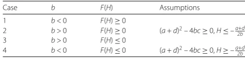
Table 1 Situations matching Theorem 3.3
Case b F(H) Assumptions
1 b< 0 F(H)≥0
2 b> 0 F(H)≥0 (a+d)2– 4bc≥0,H≤–a+d
2b
3 b> 0 F(H)≤0
4 b< 0 F(H)≤0 (a+d)2– 4bc≥0,H≥–a+d
2b
According to Lemma 3.1 and Remark 3.2,
H=H+ T
t
F(H) –F(H)ds
≤ ˆu(t) =H+ T
t
bu(s)ˆ 2+ (a+d)ˆu(s) +cds
≤λ=λ+ T
t
F(λ)ds,
thusu(t)ˆ ∈[H,λ].
(ii) can be proved similarly.
(iii) Equation (3.9) becomes a solvable and linear equation
ˆ
u(t) =H+ T
t
(a+d)ˆu(t) +cds.
It is obvious thatu(t) is bounded on [0,ˆ T].
Theorem 3.3(iii) is easy to check, but (i) and (ii) are not directly connected with the coefficients. Next, we give some equivalence conditions.
According to Vieta’s theorem, Theorem 3.3(i) equals the following two situations:
• b< 0,F(H)≥0,
• b> 0,F(H)≥0,(a+d)2– 4bc≥0,H≤–a2+bd.
Similarly, Theorem 3.3(ii) equals another two situations:
• b> 0,F(H)≤0,
• b< 0,F(H)≤0,(a+d)2– 4bc≥0,H≥–a+d
2b.
This can be a criterion to judge whether ODEs with constant-coefficient are solvable or not (see Table 1). In Table 1,
F(H) =bH2+ (a+d)H+c.
Next, we focus on the connections between Theorem 3.3 and the monotonicity condi-tions. According to Peng and Wu [5] and Wu [7], matching one of the following conditions, we can also get the well-posedness of ODEs (1.1) on [0,T].
Lemma 3.4(Monotonicity conditions) ODEs(3.8)have a unique solution if one of the following cases holds:
(i)
x y
–c –d
a b
x y
whereβ1andβ2are nonnegative constants.Whenβ1> 0,H> 0,thenβ2≥0;when β2> 0,thenβ1≥0,H≥0.
(ii)
x y
–c –d
a b
x y
≥β1|x|2+β2|y|2, (3.11)
whereβ1andβ2are nonnegative constants.Whenβ1> 0,H< 0,thenβ2≥0;when β2> 0,thenβ1≥0,H≤0.
According to Vieta’s theorem, Lemma 3.4 is equivalent to the following lemma.
Lemma 3.5(Equivalence conditions)
(i) A necessary and sufficient condition for Lemma3.4(i)is
b< 0, H> 0, (a–d)2+ 4bc< 0. (3.12)
(ii) A necessary and sufficient condition for Lemma3.4(ii)is
b> 0, H< 0, (a–d)2+ 4bc< 0. (3.13)
As can be seen in Lemma 3.5(i),
(a–d)2+ 4bc< 0.
Obviously, we have
(a+d)2– 4bc> 0,
and also,b< 0,H> 0.
IfF(H)≥0, Lemma 3.5(i) matches case 1 of Table 1; ifF(H)≤0,H≥–a–2+db, Lemma 3.5(i) matches case 4 of Table 1; ifF(H)≤0,H≤––2a+db, we must haveλ≥Hsuch thatF(λ) = 0. Thanks toH> 0, the following relation holds true:
0 = 0 + T
t
F(0) –cds
≤ ˆu(t) =H+ T
t
Fu(t)ˆ ds
≤λ=λ+ T
t
F(λ)ds.
According to Theorem 3.3, the analysis above meansu(t)ˆ ∈[0,λ]. Thus, Lemma 3.5(i) totally falls into the framework of Theorem 3.3.
An example is given where the coefficients match the assumption of Theorem 3.3. It is noted that this example does not match the monotonicity conditions.
Example1 Consider the following ODEs: ⎧
⎨ ⎩
Xt= 1 +0t(2Xs+ 2Ys)ds, Yt=12XT+tT(–3Xs+Ys)ds,
0≤t≤T, (3.14)
wherea= 2,b= 2,c= –3,d= 1,H=12.
According to Lemma 3.4, the signs ofHandbshould be different to match the mono-tonicity conditions. Thus, the well-posedness of equations (3.14) cannot be proved by us-ing the framework of monotonicity conditions.
Nevertheless, we haveb= 2 > 0, and
F(H) =bH2+ (a+d)H+c=1 2+
3
2– 3 = –1 < 0.
Then ODEs (3.14) match Theorem 3.3(ii) (case 3 of Table 1). It is obvious that ODEs (3.14) have a unique solution thanks to the analysis above.
Case 2: Functional coefficients
In this part, we consider the case where coefficients of ODEs (1.1) are functions defined on [0,T]. In this case,F(s,u(s)) takes the form (3.4), and also Assumption 2.1 holds. Itˆ is noted thatF(t,u(t))/F(t,ˆ u(t)) defined in (3.7) is regarded as an upper/lower bound ofˆ F(s,u(s)). In analogy to Theorem 3.3, we have the following result.ˆ
Theorem 3.6 Assume that Assumption2.1holds,equation(3.6)has a bounded solution y,y for arbitrary T if there exists one of the following three situations:
(i) F(t,H)≥0,andF(t,H)has a zero point in[H,∞]. (ii) F(t,H)≤0,andF(t,H)has a zero point in[–∞,H]. (iii) bs= 0.
Proof (i) The proof is the same as that of Theorem 3.3(i). As a result of
F(y)≤F(t,y)≤F(y),
we haveu(t)ˆ ∈[H,λ].
(ii) can be proved similarly, andu(t)ˆ ∈[λ,H].
(iii) Ifbs≡0, we have a positive constantC0such that
–C0[y+ 1]≤F(y)≤F(y)≤C0[y+ 1].
According to Theorem 3.3(iii), the analytic solution of the upper/lower bound equation can be derived, which means equation (3.4) has a bounded solution on [0,T].
espe-cially when ODEs (1.1) cannot match the monotonicity conditions. In the next section, the linear transformation method is used to generalize the framework of the monotonic-ity conditions.
4 The linear transformation method Consider the following homogeneous ODEs:
⎧
If equation (4.1) cannot meet the requirement of Theorem 3.3 or Lemma 3.4, consider the following transformation:
where the transformation matrixA=a11a12 a21a22 .
Substituting (4.1) into (4.2), we have
⎧
It is noted that in equations (4.3),
˜
X0=C1+C2Y˜0, C1,C2∈R.
From Wu [10], Lemma 3.4 should be adjusted to match a new form ofX˜0, whereC2is the
Lemma 4.1 ODEs(3.8)have a unique solution if one of the following cases holds:
Note that coefficients after transforming should match the following inequality to meet the requirement of the monotonicity conditions. Denotinga11/a12=m,a21/a22=n, we
have
In analogy to Lemma 3.5, Lemma 4.1 is equivalent to the following assumption.
Lemma 4.2 Lemma4.1holds if and only if one of the following two cases occurs:
(i) b˜2≤0,C2≤0,H˜ ≥0,(m–n)2(b1–f2)2+ 4f(m)f(n) < 0,
Similarly, in Lemma 4.2(ii),
In summary, we have the following result.
Theorem 4.3 On the curve of function f(x) =b2x2+ (b1–f2)x–f1,if there are two pairs
(m,f(m))and(n,f(n))matching the following criterion:
⎧
then by means of linear transformationmcnc21cc21 ,equations(4.1)match Lemma4.2,where c1,c2are constants in R.When c1/c2≤0,ODEs(4.3)match Lemma4.2(i);when c1/c2≥0,
ODEs(4.3)match Lemma4.2(ii).
In the following example, where the monotonicity conditions and regular decoupling field methods cannot be directly applied, the well-posedness of ODEs can be obtained by using the linear transformation method discussed in this section.
Example2 Consider the following linear ODEs: ⎧
According to Lemma 4.2, ODEs (4.10) cannot match the monotonicity conditions. In addi-tion, it is noted that Theorem 3.3 cannot be applied directly. Here we consider the linear transformation method to get the well-posedness of ODEs (4.10): According to Theo-rem 4.3, we need to find two points on the curvef(y) =y2– 2 which matches equation
(4.9). (4.9) is as follows:
⎧
Take two points (2, 2) and (–1, –1) which match equation (4.9), then the transformation matrixAis–1 12 1 . TakeAinto (4.3), the linear ODEs after transforming is as follows:
⎧
5 Conclusion
In this paper, we introduce two methods to solve the two-point boundary value problems of ODEs (1.1). The first method is the regular decoupling field which generates from the unified approach for FBSDEs. But for ODEs, the regular decoupling field method has a di-rect criterion which makes it easy to apply. Moreover, in this paper, it can be proved that the monotonicity conditions are a special case of the regular decoupling field method. The second method we introduce is the linear transformation method. It can be applied to cases where the monotonicity conditions and the regular decoupling field method can not. We also give examples in this paper to illustrate how these two methods develop the theory of the two-point boundary value problems for ODEs which has meaningful applications in optimal control and PDEs theory. In addition, the linear transformation method can also be generalized into stochastic cases. This provides another way to study the well-posedness of FBSDEs, which is our future research direction and has some po-tential applications.
Acknowledgements
This work was supported by the Natural Science Foundation of China (61573217), the National High-level Personnel of Special Support Program and the Chang Jiang Scholar Program of Chinese Education Ministry.
Competing interests
The authors declare that they have no competing interests.
Authors’ contributions
All authors have contributed equally in this paper. All authors read and approved the final manuscript.
Publisher’s Note
Springer Nature remains neutral with regard to jurisdictional claims in published maps and institutional affiliations.
Received: 20 September 2017 Accepted: 31 January 2018 References
1. Yong, J., Zhou, X.Y.: Stochastic controls: Hamiltonian systems and HJB equations. IEEE Trans. Autom. Control46, 1846 (1999)
2. Lakshmikantham, V., Murty, K.N., Turner, J.: Two-point boundary value problems associated with nonlinear fuzzy differential equations. Math. Inequal. Appl.4, 527–533 (2001)
3. Abbas, S., Benchohra, M., N’Guérékata, G.M.: Boundary value problems for differential equations with fractional order and nonlocal conditions. Surv. Math. Appl.71, 2391–2396 (2009)
4. Hu, Y., Peng, S.: Solution of forward–backward stochastic differential equations. Probab. Theory Relat. Fields103, 273–283 (1995)
5. Peng, S., Wu, Z.: Fully coupled forward–backward stochastic differential equations and applications to optimal control. SIAM J. Control Optim.37, 825–843 (1999)
6. Yong, J.: Finding adapted solutions of forward–backward stochastic differential equations: method of continuation. Probab. Theory Relat. Fields107, 537–572 (1997)
7. Wu, Z.: One kind of two point boundary value problems associated with ordinary differential equations and application. J. Shandong Univ. Nat. Sci.32, 16–23 (1997)
8. Ma, J., Wu, Z., Zhang, D.T., Zhang, J.F.: On well-posedness of forward–backward SDEs—a unified approach. Ann. Appl. Probab.25, 2168–2214 (2015)
9. Zhang, J.F.: The wellposedness of FBSDEs. Discrete Contin. Dyn. Syst., Ser. B6, 927–940 (2006)