Permanence and global stability of a May cooperative system with strong and weak cooperative partners

R E S E A R C H

Open Access

Permanence and global stability of a May

cooperative system with strong and weak

cooperative partners

Liang Zhao

_{, Bin Qin}

_{and Fengde Chen}

*_{Correspondence:}

[email protected]

1_{College of Information and}

Statistics, Guangxi University of Finance and Economics, Nanning, P.R. China

Full list of author information is available at the end of the article

Abstract

In this paper, a May cooperative system with strong and weak cooperative partners is proposed. First, by using differential inequality theory, we obtain the permanence and non-permanence of the system. Second, we discuss the existence of the positive equilibrium point and boundary equilibrium point, after that, by constructing suitable Lyapunov functions, it is shown that the equilibrium points are globally

asymptotically stable in the positive octant. Finally, examples together with their numerical simulations show the feasibility of the main results.

MSC: 34C05; 34C25

Keywords: Cooperative system; Strong; Weak; Global stability

1 Introduction

Cooperative system is an important system in the field of biology, and the importance of the system is the same as for prey–predator and competitive systems. Many scholars have done research on the cooperative ecosystem (see [1–12]). May [1] described a cooperative system with the following equations:

dx1

dt =r1x1

1 – x1

a1+b1x2 –c1x1

,

dx2

dt =r2x2

1 – x2

a2+b2x1 –c2x2

,

(1.1)

wherex1,x2are the densities of the speciesx1,x2at timet, respectively,rirefers to the intrinsic rate of populationxi,i= 1, 2, andbi,i= 1, 2, refers to the coefficients of cooper-ation,ri,ai,bi,ci,i= 1, 2 are positive constants. His research shows that the cooperative system has a unique positive equilibrium point and it is globally asymptotically stable.

Cui and Chen [2] think that a non-autonomous form is more reasonable. They put for-ward the following cooperation system:

dx1

dt =r1(t)x1

1 – x1

a1(t) +b1(t)x2

–c1(t)x1

,

dx2

dt =r2(t)x2

1 – x2

a2(t) +b2(t)x1

–c2(t)x2

,

(1.2)

where the functionri(t),ai(t),bi(t),ci(t),i= 1, 2 are continuous functions and bounded above and below by positive constants. Under the premise of ri(t), ai(t), bi(t), ci(t),

i= 1, 2 are periodic function, they get the sufficient conditions which guarantee the global asymptotic stability of positive periodic solutions of this system.

In view of the influence of time delay, species interactions and feedback, Chen, Liao and Huang [3] proposed the followingn-species cooperation system:

dxi(t)

dt =ri(t)xi(t)

1 – xi(t)

ai(t) +

n

j=1,j=ibij(t)

0

–TijKij(s)xj(t+s)ds

–ci(t)xi(t)

–di(t)ui(t)xi(t) –ei(t)xi(t)

0 –τi

Hi(s)ui(t+s)ds,

dui(t)

dt = –αi(t)ui(t) +βi(t)xi(t) +ri(t)

0 –ηi

Gi(s)xi(t+s)ds,

(1.3)

wherexi(t),i= 1, . . . ,nis the density of cooperation speciesXi,ui(t),i= 1, . . . ,n, is the feed-back control variable. The authors obtained the sufficient conditions which guarantee the permanence by using differential inequality theory. For more work as regards the system, we can refer to [4–6].

In the real world, individual organisms are associated with a strong and weak differential. Mohammadi [13] proposed a Leslie–Gower predator–prey model:

dH1

dt = (r1–bH1–αH2)H1, dH2

dt = (αH1–c1–c2P)H2, dP

dt =

r2–

a2P

H2

P,

(1.4)

wherer1,b1,α,c1,c2,r2,a2are positive constants, the predators can distinguish between strong and weak prey and predator eats only weak prey, when a prey becomes weak, it does not become strong again; by constructing a suitable Lyapunov function, it is shown that the unique equilibrium point is stable in the positive octant.

Conversely, in many cooperative ecosystems, partners like strong partners, because the strong partners are more conducive to their survival. This shows that the cooperative ob-ject should only be part instead of the whole.

There are two populations:

The partnerH, whose total density isH, is divided into two categoriesH1,H2.H1 de-notes the strong partner density andH2denotes the weak. Of the other partner, the total density isP.

The May cooperative model (1.1) is our basic model and we consider the following as-sumptions to improve the model:

(A1) The partnerPcan distinguish between strong partnerH1and weak partnerH2and

the partnerPcooperates only with strong partnerH1.

(A2) When provided with food resources, the weak partnerH2has no negative influence

(A3) Due to the lack of sufficient food resources, once it becomes weak, the weak partner

H2and their descendants will no longer be strong.

(A4) The rate of becoming weak is described by the simple mass actionαH1H2. By the above assumptions, we propose a model as follows:

dH1

dt =r1H1

1 – H1

a1+b1P

–c1H1– αH2

r1

,

dH2

dt =H2(αH1+d–eH2), dP

dt =r2P

1 – P

a2+b2H1 –c2P

,

(1.5)

whereri,ai,bi,ci,d,i= 1, 2 are positive constants.

The structure of this article as follows. In Sect. 2 we will introduce several useful lemmas and prove permanence and non-permanence. In Sect. 3 we will discuss the existence of the equilibrium point. In Sect. 4 global stability of equilibrium points is studied. In Sect. 5 two examples are given to show the feasibility of our results. We end this paper by a brief discussion.

2 Permanence and non-permanence

In view of the actual ecological implications of system (1.5), we assume that the initial valueHi(0) > 0,i= 1, 2,P(0) > 0 in system (1.5). Obviously, any solution of system (1.5) remains positive for allt≥0.

Lemma 2.1(see [14]) Let a> 0,b> 0.

(I) If dx

dt ≥x(b–ax),thenlim inft→+∞x(t)≥ b

afort≥0andx(0) > 0.

(II) If dx_dt ≤x(b–ax),thenlim sup_t→+∞x(t)≤b_afort≥0andx(0) > 0.

Lemma 2.2(see [15]) Let a> 0,b> 0.

Ifdx_dt ≤x(–b–ax),thenlimt→+∞x(t) = 0for t≥0and x(0) > 0.

Theorem 2.1 If the assumptions(B1)and(B2)hold,

(B1) M= 1 –α_r1d_e> 0, (B2) 1 > α

2_(a 1c2+b1)

r1e(a1c1c2+b1c1+c2),

then system(1.5)is permanent.

Proof Let (H1(t),H2(t),P(t))T be any positive solution of system (1.5), from the second equation of system (1.5), it follows that

dH2

dt ≥H2(d–eH2).

According to Lemma 2.1, we have

lim inf

t→+∞ H2(t)≥ d e

def

For any positive constantεsmall enough, it follows from (2.1) that there exists a large enoughT1> 0 such that

H2(t) >H2i–ε, t≥T1. (2.2)

From the third equation, we have

dP

dt ≤r2P(1 –c2P).

According to Lemma 2.1, we have

lim sup

t→+∞ P(t)≤

1

c2 def

=Ps> 0. (2.3)

For any positive constantεsmall enough, it follows from (2.3) that there exists a large enoughT2>T1such that

P(t)≤Ps+ε, t≥T2. (2.4)

By applying (2.2) and (2.4), from the first equation of system (1.5), we have

dH1

dt ≤r1H1

1 – H1

a1+b1(Ps+ε)

–c1H1– α(Hi

2–ε)

r1

, t≥T2.

According to Lemma 2.1, we have

lim sup

t→+∞ H1(t)≤

1 –α(H i

2–ε)

r1

a1+b1(Ps+ε) 1 +a1c1+b1c1(Ps+ε)

.

Lettingε→0 and by applying (2.1) and (2.3)

lim sup

t→+∞

H1(t)≤

a1c2+b1

a1c1c2+b1c1+c2

Mdef=H₁s> 0. (2.5)

For any positive constantεsmall enough, it follows from (2.5) that there exists a large enoughT3>T2such that

H1(t)≤H1s+ε, t≥T3. (2.6)

Then the second equation of (1.5) leads to

dH2

dt ≤H2 α H

s

1+ε

+d–eH2

, t≥T3.

According to Lemma 2.1, we have

lim sup

t→+∞

H2(t)≤ α(Hs

1+ε) +d

Lettingε→0 in the above inequality leads to

lim sup

t→+∞

H2(t)≤

αH1s+d

e

def

=H₂s. (2.7)

For any positive constantεsmall enough, it follows from (2.7) that there exists a large enoughT4>T3such that

H2(t)≤H2s+ε, t≥T4. (2.8)

Then substituting (2.8) into the first equation of (1.5), we have

dH1

dt ≥r1H1

1 –H1

a1

–c1H1– α(Hs

2+ε)

r1

, t≥T4.

According to Lemma 2.1, we have

lim inf

t→+∞ H1(t)≥

1 –α(H s

2+ε)

r1

a1

a1c1+ 1 .

Lettingε→0 and by applying (2.5) and (2.7)

lim inf

t→+∞ H1(t)≥M– α2Hs

1

r1e def

=H₁i> 0. (2.9)

From the third equation of system(1.5), it follows that

dP dt ≥r2P

1 – P

a2 –c2P

.

According to Lemma 2.1, we have

lim inf

t→+∞ P(t)≥

a2

a2c2+ 1 def

=Pi. (2.10)

(2.1), (2.3), (2.5), (2.7), (2.9) and (2.10) show that if the assumptions (B1), (B2) hold, then

system (1.5) is permanent.

Theorem 2.2 If the assumption(B3)holds, (B3) M= 1 –α_r1d_e< 0,

then the weak partners H2and partners P are permanent,the strong partners H1are

non-permanent.

Proof Let (H1(t),H2(t),P)Tbe any positive solutions of system (1.5) fort≥0. From the proof Theorem 2.1, we know

dH1

dt ≤r1H1

1 – H1

a1+b1(Ps+ε)

–c1H1–

α(H₂i–ε)

r1

, t≥T2.

Noting that condition (B3) implies that 1 –

α(Hi

2–ε)

According to Lemma 2.2, we have

lim

t→+∞H1(t) = 0. (2.11)

By applying (2.11), from the second equation of system (1.5), it is easy to prove that

lim

t→+∞H2(t) = d

e. (2.12)

(2.3), (2.10), (2.11) and (2.12) show that if the assumptions (B3) hold, then the weak part-nersH2and partnersPare permanent, the strong partnersH1are non-permanent.

3 Existence of equilibrium point

Theorem 3.1 If the assumption(B1)holds,then system(1.5)have a unique positive

equi-librium point.

Proof We determine the positive equilibrium of the system (1.5) through solving the fol-lowing equations:

⎧ ⎪ ⎨ ⎪ ⎩

1 – H1

a1+b1P–c1H1–

αH2

r1 = 0, αH1+d–eH2= 0,

1 –_a2+P_b

2H1 –c2P= 0.

(3.1)

Here we transform Eqs. (3.1) into the following form:

⎧ ⎪ ⎨ ⎪ ⎩

1 – H1

a11+b11P–c11H1= 0, 1 –_a2+P_b

2H1 –c2P= 0, αH1+d–eH2= 0,

(3.2)

wherea11=Ma1,b11=Mb1,c11= (c1+_rα₁d_e)/M, from the first and second equations of (3.2), we have

DH₁2+EH1+F= 0, (3.3)

where

D=b2(a11c11c2+b11c11+c2), F= –a11(a2c2+b2+ 1),

E=(a2c2+ 1) +c11(a11+a11a2c2+a2b11) –b2(a11c2+b11)

.

From the termsDandFof (3.3), we know that there is a unique positive solutionsH₁∗. SubstituteH₁∗into the second and third equations of (3.1). Then system (1.5) has a unique

positive equilibrium pointE1(H1∗,H2∗,P∗).

4 Global stability

Theorem 4.1 If the assumptions(B1)and(B4)hold, (B4) α2<_aa₂₊2r_b1₂c1_Hes

1,

then the positive equilibrium of system(1.5)is globally asymptotically stable.

LetA(t)def= _(a1+b 1

Note first that both of the off-diagonal elements of matrixAare negative and

η1η2r1r2– wheredL_dt = 0. According to the Lyapunov asymptotic stability theorem [9], the equilibrium point (H₁∗,H₂∗,P∗) is globally asymptotically stable in the interior ofR3

+. This completes the

proof.

Theorem 4.2 If the assumptions(B3)and(B5)hold, (B5) α2<r1c1e,

Proof We defineL:{(H1,H2,P)∈R3+:H1> 0,H2> 0,P> 0} →Rby

Note first that both of the off-diagonal elements of matrixAare negative and

Noting thatab≤θa₂2 +b_2θ2,θ> 0, from (2.11), for sufficiently small constantε0> 0, there wheredL_dt = 0. According to the Lyapunov asymptotic stability theorem [9], the equilibrium point (0,H2∗,P∗) is globally asymptotically stable in the interior ofR3+. This completes the

proof.

5 Example and numeric simulation

Consider the following system:

Figure 1Dynamical behavior of system (5.1) with initial values (0.4, 1.2, 0.7)T_{, (0.1, 0.8, 0.2)}T_{and (0.25, 0.6, 0.3)}T

Consider the following system:

dH1

dt = 3H1

1 – H1

2 + 2P– 2H1–

3.5H2 3

,

dH2

dt =H2(3.5H1+ 2 – 2H2), dP

dt = 2P

1 – P

2 + 0.8H1 – 1.5P

.

(5.2)

By calculation, we haveM= 1 – _rαd

1e = –0.1 < 0,α

2_{= 10.89 <} a2r1c1e

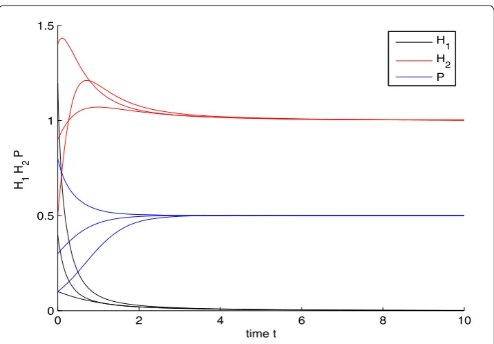
a2+b2H1s = 12, it is easy to see that the conditions (B3) and (B5) are verified. It follows from Theorem 3.1 that there is a unique positive equilibrium point (H1∗,H2∗,P∗) = (0, 1, 0.5) of system (5.2) and it is

globally asymptotically stable. Our numerical simulation supports our result (see Fig. 2).

6 Discussion

In this paper, a May cooperative system with strong and weak cooperative partners is studied. We obtained the sufficient conditions that guarantee the permanence, non-permanence and the global stability of the equilibrium points. By comparing the condi-tions of (B1) and (B3), we found that asαbecomes larger and larger, the strong partner changes from persistent to extinct. The ecological explanation is that more and more the strong partner become a weak partner, thus we have extinction of the strong. The above numerical simulations also supports this conclusion.

Figure 2Dynamical behavior of system (5.2) with initial values (0.4, 1.4, 0.8)T_{, (0.1, 0.9, 0.3)}T_{and (1.2, 0.5, 0.1)}T

Acknowledgements

The research was supported by Guangxi College Enhancing Youth’s Capacity Project (2017KY0599) and the Scientific Research Development Fund of Young Researchers of Guangxi University of Finance and Economics (2017QNB18).

Competing interests

The authors declare that there is no conflict of interests.

Authors’ contributions

All authors contributed equally to the writing of this paper. All authors read and approved the final manuscript.

Author details

1_{College of Information and Statistics, Guangxi University of Finance and Economics, Nanning, P.R. China.}2_{College of}

Mathematics and Computer Science, Fuzhou University, Fuzhou, P.R. China.

Publisher’s Note

Springer Nature remains neutral with regard to jurisdictional claims in published maps and institutional affiliations.

Received: 9 January 2018 Accepted: 2 May 2018

References

1. May, R.M.: Theoretical Ecology, Principles and Applications. Sounders, Philadelphia (1976)

2. Cui, J.A., Chen, L.S.: Global asymptotic stability in a nonautonomous cooperative system. Syst. Sci. Math. Sci.6(1), 44–51 (1993)

3. Chen, F.D., Liao, X.Y., Huang, Z.K.: The dynamic behavior of N-species cooperation system with continuous time delays and feedback controls. Appl. Math. Comput.181(2), 803–815 (2006)

4. Chen, L.J., Xie, X.D.: Permanence of an N-species cooperation system with continuous time delays and feedback controls. Nonlinear Anal., Real World Appl.12(1), 34–38 (2011)

5. Nasertayoob, P., Vaezpour, S.M.: Permanence and existence of positive periodic solution for a multi-species cooperation system with continuous time delays, feedback control, and periodic external source. Adv. Differ. Equ.

2012(1), Article ID 156 (2012)

6. Muhammadhaji, A., Teng, Z.D., Abdurahman, X.: Permanence and extinction analysis for a delayed ratio-dependent cooperative system with stage structure. Afr. Math.25(4), 897–909 (2014)

7. Li, Z., Han, M.A., Chen, F.D.: Influence of feedback controls on an autonomous Lotka–Volterra competitive system with infinite delays. Nonlinear Anal., Real World Appl.14(1), 402–413 (2013)

8. Leon, C.V.D.: Lyapunov functions for two-species cooperative systems. Appl. Math. Comput.219(5), 2493–2497 (2012) 9. Yang, K., Miao, Z.S., Chen, F.D., Xie, X.D.: Influence of single feedback control variable on an autonomous Holling-II

type cooperative system. J. Math. Anal. Appl.435(1), 874–888 (2016)

11. Xie, X.D., Miao, Z.S., Xue, Y.L.: Positive periodic solution of a discrete Lotka–Volterra commensal symbiosis model. Commun. Math. Biol. Neurosci.2015, Article ID 2 (2015)

12. Wu, R.X., Lin, L., Zhou, X.Y.: A commensal symbiosis model with Holling type functional response. J. Math. Comput. Sci.16, 364–371 (2016)

13. Mohammadi, H., Mahzoon, M.: Effect of weak prey in Leslie–Gower predator–prey model. Appl. Math. Comput.

224(4), 196–204 (2013)

14. Chen, F.D.: On a nonlinear nonautonomous predator–prey model with diffusion and distributed delay. Comput. Appl. Math.180(1), 33–49 (2005)