Location based distributed sleeping cell detection and root cause analysis for 5G ultra dense networks

R E S E A R C H

Open Access

Location-based distributed sleeping cell

detection and root cause analysis for 5G

ultra-dense networks

Sergio Fortes , Raquel Barco

and Alejandro Aguilar-Garcia

Abstract

The sleeping cell problem is one of the most critical issues for cellular deployments, consisting in the outage of a cellular station, which, conversely, works properly from the point of view of the monitoring system. This problem is often not detectable by the operators, and it could lead to severe degradations in the service provision in the long term. This issue has been commonly managed by the centralized analysis of network performance indicators. However, those solutions are unsuitable for the new ultra-dense small cell scenarios that will characterize 5G deployments. New approaches are required to cope with the high level of cell overlapping as well as the huge number of sites to be managed. In this context, a novel mechanism to detect sleeping cell issues is proposed, which takes advantage of the recent advances in indoor localization as well as monitoring data obtained by user equipments. In addition, a root cause analysis of the cell failure is presented. The capabilities of the proposed approach are evaluated in a realistic key scenario, showing the feasibility and usefulness of the proposed location-based approach.

Keywords:Self-organizing networks (SON), 5G, DenseNets, Small cell, Localization, Self-healing, Sleeping cell, Troubleshooting, Detection

1 Introduction

Current studies on 5G focus on three main objectives:

converged fiber-wireless, super-efficient, and super-fast

mobile networks [1]. To achieve the last two objectives, 5G networks are expected to hugely increase network densification. For these, the ultra-dense deployment of

small cells or DenseNets (with a few tens of meters inter-site distance) will be one of the main approaches used to reach the upcoming coverage and throughput requirements [2]. Small cells consist on low-powered, low-range base stations (BSs) used to cover especially difficult radio locations, as well as to increase network capacity for specific hotspots. Small cells are already started to become a common approach to provide coverage in-doors (e.g., malls or offices) or to shadowed locations. They are also employed to serve high demanding spots (e.g., airports, stadiums, etc.). Different small cell models have been defined for indoor scenarios, such aspicocells, i.e., cells with up to 200-m coverage, and femtocells, i.e.,

cells with coverage in the range of tens of meters and making use of broadband non-dedicated infrastructure, e.g., digital subscriber line (DSL), to connect with the op-erator’s network [3].

The large number of small cells, together with the grow-ing coexistence of multiple radio access technologies (RATs) like global system for mobile communications (GSM), universal mobile telecommunications system (UMTS), long-term evolution (LTE), etc., leads to an increasing complexity in the operations, administration, and management (OAM) of cellular networks. In order to overcome this complexity, the Next Generation Mobile Networks (NGMN) Alliance and the 3rd Generation Partnership Project (3GPP) introduced the concept of self-organizing networks (SON), which aims to automate the OAM procedures [4], reducing costs and increasing the network performance and quality of service. SON en-compasses three main categories:self-configuration, which is related to the capability of automatically deploying new elements in a network andself-optimization, on the ability of the network to adapt to changing service requirements. * Correspondence:[email protected]

Universidad de Málaga, Andalucía Tech, Departamento de Ingeniería de Comunicaciones, Campus de Teatinos s/n, 29071 Málaga, Spain

Finally, self-healing covers the tasks related to failure management and prevention.

This work is focused on the self-healing functionalities for ultra-dense small cell networks. Self-healing is key for network OAM automation and performance, since network failures can lead to service degradations that might highly impact the brand image and the long-term revenue of operators. Failure management is divided in four main subtasks [5]. Firstly, detectionconsists in the discovery of network problems, i.e., identifying cells with degradations in the provided service. Secondly, diagno-sis, also called root cause analysis, aims at identifying the specific cause or fault producing the degradation. Finally, once a problem has been detected, different actions can take place tocompensateits effects until re-coveryactions restore the network to its full functional-ity. In classic failure management approaches, these are very time consuming and signaling generating tasks. This makes the automation of these functions a field attracting an increasing attention, where the implica-tions of its application for 5G scenarios have been only scarcely considered.

Moreover, one of the most common problems in small cell scenarios is thesleeping cellissue, which is the situ-ation where a base stsitu-ation is not able to properly serve users, and this is not directly reflected in the OAM monitoring indicators [6]. The causes behind this prob-lem range from BS unplugging, failures in the cell hard-ware, or incorrect configuration. Since many of these fault causes behind the sleeping cell issue could be quickly compensated and/or recovered with automatic actions (like restarting the BS or updating its software), fast mechanisms for failure detection/diagnosis are essen-tial to automatically trigger those tasks. Therefore, detec-tion and diagnosis should, ideally, identify the failure and its causes in the range of minutes/seconds.

However, small cells can be particularly prone to failures (due to its more accessible hardware, use of non-dedicated backhaul, etc.) and have limited reporting capabilities and reduced coverage areas which very variable level of use. Therefore, it is common that not alarm or clear perform-ance degradation might be reported to the OAM system in these situations.

Instead, user equipment (UE) positioning informa-tion can serve as an addiinforma-tional input for troubleshoot-ing of these issues. For example, the knowledge on UEs location is becoming growlingly available in both outdoor and indoor scenarios [7]. Localization mech-anisms based on the small cell deployments [8] open the door to using location to support the OAM tasks. Even if its use for self-healing in indoor scenarios has been just recently proposed [9], its usefulness has been previously demonstrated for macrocell scenarios and other OAM tasks (e.g., for coverage optimization [10]).

Also, another important limitation of classical approaches is the high signaling costs of transmitting the monitoring data to the centralized OAM/SON systems, which might overload the operator’s network. Additionally, 5G services and the operation of dense small cell deployments will also impose very demanding response time and computational requirements when performed in a centralized manner. In order to avoid these problems, SON mechanisms should be as automatic and distributed as possible, avoiding the satur-ation of the network and the centralized OAM elements.

Taking all this into account, the present work defines a novel fully distributed and automated location-based mechanism for sleeping cell detection and cause diagno-sis in ultra-dense scenarios based on the deployment of small cells. Here, the required UE locations are assumed to be provided by external localization sources. The de-tails of the particular method used for UE localization are considered outside the scope of the detection/diag-nosis algorithm, making it agnostic to the use of any localization source. Hence, this paper is organized as fol-lows: Section 2 discusses the challenges and state of the art in location-based mechanisms and detection and diagnosis of sleeping cell issues for the considered small cells scenario. Section 3 summarizes the characteristics and assumptions for location-based processing of moni-toring information. The proposed mechanisms for detec-tion and cause analysis are detailed in secdetec-tions 4 and 5, respectively. The combined distributed scheme is then described in Section 6. The defined system is evaluated in Section 6 and the conclusions of this study are finally presented in Section 7.

2 Related work

Classic self-healing macrocell solutions [11] are unsuit-able for small cell deployments due to multiple reasons. Firstly, small cells provide reduced monitoring functions in comparison to their macrocell counterparts, as a re-sult of their limited computing capabilities and in order to avoid backhaul saturation. Secondly, general network performance indicators might not be highly affected by the cell failure, making the issues to remain undetected for long periods of time. This is mainly due to the occa-sional low number of UEs in the affected area. Also, be-cause most of the UEs that should be served by the faulty cell might be covered by neighboring BSs (given the high level of coverage overlapping between cells in dense small cell environments). Only when there are users in spots that are poorly covered by other cells or if the ser-vice demand is high (because there are a large number of users or they require high capacity), the failure of one BS may be detected by classic network performance indica-tors (e.g., call dropping ratio).

the UEs, such as drive tests, UE app monitoring, or ana-lysis of the control plane messages. In order to overcome limitations of drive tests (classically performed by field en-gineers with especial terminals), recent standardization work has established mechanisms for minimization of drive test (MDT). In MDT, measurements automatically gathered from common terminals are used for network monitoring. In this way, the work presented in [6] is based on the use of MDT information for sleeping cell detec-tion. However, MDT is typically applied in outdoor en-vironments where the terminals’ reports are combined with geographical information obtained from satellite or cellular-based localization (e.g., based on observed time difference of arrival (OTDoA)). Thus, those systems have very low performance indoors due to the lack of satellite coverage and the short distance between cells.

Following a different approach, the work in [12] proposed a system that performs particle filtering for detection of sleeping cells. This is applied in a distributed manner based on UE measurements. However, this method required the use of large databases of previous measurements. Also, po-sitioning information was not used and no diagnosis ana-lysis or the conditions of implementing the distributed algorithm were addressed.

UE localization systems are increasingly available in in-door scenarios, based on multiple technologies under development or already commercialized. These are often based on the analysis of the received signal characteristics (e.g., time of arrival, received power, etc.) from different systems such as radio-frequency identification (RFID) [13], WiFi [14], cellular [8], and ultra-wideband (UWB) [15]. Although the use of UE localization has already attracted interest in other OAM tasks, e.g., for the pre-sented MDT cases, it has been mainly neglected in previous self-healing works and particularly for indoor scenarios.

Therefore, up to our knowledge, none of the previous works presented a consistent fast and distributed detec-tion/diagnosis mechanism for sleeping cell issues in dense scenarios. Equally, previous developments did not take advantage of automatically obtained location infor-mation for self-healing.

In this respect, the present work presents three main contributions. Firstly, it defines a location-based mechan-ism for sleeping small cell detection. Secondly, it establishes the general architecture, procedures and restrictions for a distributed implementation of the mechanism in Dense-Nets. Thirdly, it also proposes a system for the distributed analysis of the root cause behind the sleeping cell issue.

3 Location and radio information application 3.1 UE radio measurements

In the proposed approach, UE measurements are estab-lished as the main source of information for detection, instead of the classical approach based on centralized

data coming from the OAM system. In particular,received signal strength(RSS) measurements are chosen as the in-put for the mechanisms. RSS is defined as the received power level from the base station downlink reference sig-nals. The use of RSS values has multiple advantages over other indicators. Firstly, they are not event oriented, i.e., they can be obtained by the terminal at any time/position, not only in connected mode but also in idle mode. Sec-ondly, in comparison to signal quality indicators such as the call blocking ratio (CQI), RSS values are not affected by the variable interference conditions, which are also very dependent on the network load (especially for the LTE case). Thirdly, regarding practical implementation aspects, radio analysis Android apps (e.g., G-NetTrack [16]) provide the RSS measured values, whereas they do not present quality indicators for most commercial terminals [16]. This is especially important not only from a proto-type point of view but also for the possible over-the-top user-level implementations of the proposed system, which could be adopted in some scenarios (e.g., if the monitoring function is combined with a navigation application in-stalled in the smartphones).

Even though the integration between user-level apps and the cellular management plane could be not straight-forward, recent works indicate a trend towards an increas-ingly tighter integration between them. In this respect, the work in [9] proposed the interfaces and architecture re-quired to integrate app-level information into the 3GPP management plane. Meanwhile, the work in [17] devel-oped a real testbed prototype of such UE-level app based network troubleshooting. Also, end-to-end analysis and UE-level service-performance measurements are becom-ing common for network operators [18]. Moreover, the in-tegration user-level apps with the cellular management plane would become even more achievable if particular apps (such as localization applications based on the cellu-lar signal analysis) or application programming interfaces (APIs) are provided/commercialized by the operators themselves.

Fourthly, RSS-based indicators are defined for any existent RAT and they will also be established for any future 5G standard. For example in UMTS, RSS values correspond to the common pilot channel (CPICH) re-ceived signal code power (RSCP) [19], meanwhile in LTE/LTE-A, the equivalent measurement is the reference signal received power (RSRP) [20].

RSS values can be sometimes measured concurrently for both the serving and the neighboring cells. However, that is not always the case in live scenarios because the reception of neighboring cells RSS values is conditioned by multiple issues:

included in the serving neighbor cell list. That list might be incomplete, especially in UMTS. In that technology, the neighbor list is typically manually configured. Also the serving cell may require to directly receive power from each neighbor in order to keep it in the list.

Unavailability to obtain neighbor cell received power from the monitoring application: if the application used to obtain the RSS values is a user-level app (e.g., Android or iOS), the majority of commercial terminals only report the values for the serving cell [16]. Randomness on the neighboring cell UE reporting

period: even at control and radio-link monitoring level, the neighboring cells are often measured with reduced periodicity or only associated with certain events.

For these reasons, the availability of neighboring cell RSS is not guaranteed. Therefore, and in order to develop widely applicable mechanisms, only serving cell RSS values are considered available and used as inputs for the algorithm.

In addition to the UE measurements, it is assumed that UE positions are available to the SON system as part of the information provided by indoor positioning systems. The required architectural coordination of differ-ent localization sources with SON mechanisms has been presented in [9]. In this way, UEs positioning information can be obtained indistinctively from the UEs or external sources, such as surveillance camera localization.

3.2 Location-based measurements processing

In order to support efficient methods for the detection and diagnosis of sleeping cells, the combination of the presented UE RSS measurements with positioning data is proposed. Traditionally, key performance indicators (KPIs) were calculated based on statistical analysis of UE measurements and events. With that aim, the UE RSS-based indicators are computed for each cell by generat-ing statistics of the set of multiple measurementsMj[t], captured from a specific set of terminals (e.g., typically those served by a specificcellj) during a particular period of time t. The calculation is commonly performed peri-odically, e.g., one KPI value generated every hour based on the measurements gathered during that period.

Conversely, in the location-based proposed method, the individual RSS measurements gathered from the ter-minals are processed to include UE position information to generate the KPIs. Multiple solutions are possible for the integration of the positioning data with the UE RSS measurements, adapting those previously applied in other fields, especially on image processing, e.g., spatial correlation, pattern-based analysis, etc. For example, the work in [17] presented a system based on the correlation between each individual UE received levels and the

expected values given their position. Such kind of ap-proaches can be valid in femtocell environments where only a few UEs are analyzed. However, the need to pur-sue fast and computationally low cost methods where large number of UEs is present leads to the choice of

sample weights [21] for the generation of the indicators involved in the diagnosis. Although sample weights are commonly used in fields like social polling, up to our knowledge, it has only been applied in cellular networks for centralized diagnosis [22], and not for detection.

Using sample weights, the statistical relevance of each sample is potentiated depending on the expected impact of the failure in its measurement spot. Each sth RSS value is therefore assigned with a different weight, wcelli

AOI

γxyz½ s

, based on the value of the weight functionwcelli

AOI

γxyz

for the positionγxyz[s] where it was measured. In

the proposed approach, wcelli

AOI γxyz

is defined for a cer-tain area of interest (AOI) of the analyzed celli, e.g., its expected coverage area.

For any particular deployment, a set of multiple areas of interest, AOI can be established, where AOI∈ AOI.

Each of the AOIs implies a particular wcelli

AOI γxyz

and

therefore different location-based KPIs. These are used as the inputs for the detection of issues in different cells. The specific definition of these AOIs and weights is fur-ther analyzed in subsections 3.A and 3.C, respectively.

It has to be noticed that previous uses of the term AOI refer to a delimited geographical of a cellular de-ployment defined by engineers to characterize during a performance study. These often have an extension of several kilometers. In the proposed approac,h however, the AOIs imply the different set of areas from where the UE measurements are considered in the statistics calcu-lations used by the sleeping cell detection algorithm, be-ing automatically generated for each small cell, and having a much reduce size (a few meters).

In the classic non-location-based solutions, two main statistics are commonly applied for OAM purposes: the RSS mean and the RSS 5th percentile. Their classic expres-sions are therefore adapted in this approach in order to use of location-based weight samples, as described below:

Location-based RSS_mean,RSS celli_AOI cellj;t

periodtby the UEs located in the AOI of celli. |Mj[t]|

in-dicates the number of values in the set. wcelli

AOI γxyz½ s

represents the individual weight applied to one measure-ment mRSS[s], depending on the coordinates where the

sample was measuredγxyz[s]. Finally,EWis the sum of all

the applied weights,EW¼

XjMj½ tj s¼1 w

celli

AOI γxyz½ s

.

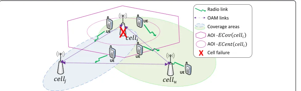
The serving celljcan be equal to cellior a

different cell of the scenario. When different, it means that the generated indicator includes information on the UEs served by celljbut

located in an AOI of celli, as presented in Fig.1.

This is one of the main characteristics of the proposed approach, as it allows the monitoring of a possible faulty celliby its neighbors. In this way, the

detection of the sleeping cell is done from the measurements obtained from its neighboring cells served UEs.

Location-based RSS_5th percentile, calculated as the RSS value below which the 5 % of the lowest collected RSS values are. For non-location approaches, this is a common indicator of the values gathered in the edges and/or at far distance of the cell as well as from low covered (shadow) spots. If a cell is in outage, the classicRSS_5th percentileof their neighboring cells would especially reflect the RSS received by the UEs more poorly served in the area originally covered by the faulty cell.

For the location-based approach and similarly to the

RSS_mean, the fifth percentile indicator is based on the

Mj[t] measurements located in a specific AOI of celli. To compute it, the common procedure for percentile calculation [23] is adapted to the use of weight samples. In this way, Mj[t], the set of RSS samples in a period, is sorted from minimum value to maximum. Then, each

sample in the position n of the ordered list Mord_j ½ t is assigned with theordinal rank rncalculated as:

rn¼

100 E_Mord

j ½ t

j j En−

wcelli

AOI γordxyz½ n

2

0 @

1

A_; ð2Þ

where wcelli

AOI γordxyz½ n

is the weight assigned to the RSS value in the position n of the ordered list, where n≤

Mord_j ½ t

¼Mj½ t. En is the partial sum of all weights applied to the ordered samples 1 to n, En¼

Xn

s¼1w celli

AOI γ ord xyz½ s

. The fifth percentile would be the sample withrn= 5. If no measurement hasrn= 5, the or-dered samples with directly inferior rk and directly su-perior rk+ 1 nearest rank are selected, in a way thatrk< 5 <rk+ 1. The correspondent RSS samples, mord_RSS½ k and

mord_RSS½kþ1 are then used to obtain the fifth percentile by linear interpolation:

RSS5thcellAOIi cellj;t

¼mord_RSS½ þk 5−rk rkþ1−rk

mord_RSS½ k−mord_RSS½kþ1

;

ð3Þ

3.3 Sample weights and AOIs for the detection of sleeping cells

In the definition of the AOIs and the sample weights

functionwcelli AOI γxyz

,different approaches can be applied

to reflect the relevance of a particular location, γxyz, in respect to a possible failure in any celli. For the sleeping cell issue, it is expected that the areas most impacted by the possible fault would be those contained in the cover-age area of celli, as it would be populated by UEs most affected by its failure.

The AOIs are therefore geographically defined in order to restrict the samples considered in each location-based indicator. Two different AOIs per cell are envisaged as alternative approaches (with different level of filtering) for the detection of the sleeping cell issue:

Expected coverage area (ECov) of the possible sleeping cell. The UEs in this area are most likely to be impacted by the cell issue. However, depending on the range of overlapping between cells, this might be compensated by the coverage coming from neighbors BSs

Expected center area (ECent) of the cell refers to locations in the core of the coverage area of a cell. In these, the signal of the cell is clearly predominant in respect to its neighbors.

Additionally, to avoid the effect generated by the macro-cell and the UEs outside the area of the indoor scenario, only the terminals inside the analyzed indoor scenario (e.g., building) are considered as inside the AOIs.

Due to the difficulty of obtaining reliable information about the specific height of the terminals and the com-plexity that would introduce a continuous vertical dimen-sion, coverage areas are commonly defined as multiple two-dimensional layers (e.g., one per building floor). In this way, γxyz= (x,y,z=ζ) represents a point in the two-dimensional Euclidean space E2 of the analyzed plane/ floor ζ. Following the same approach, the AOIs are de-fined as two-dimensional, (x,y)∈E2, for each floor of the deployment. Given this and for simplicity, the following AOI definitions would be described

These expected coverage areas can be defined in terms of signal quality (e.g., CQI-based). However, pure RSS-based definitions are preferred as justified in Section 3.A. Based on the expected received power RSS^ ððx;y;zÞ;celliÞ,

the AOI ECent(celli) is defined as:

ECent cellð iÞ ¼ ðx;yÞ∈E2

whereΔRSScentis the additional power (in dB) to be

re-ceived in the point (x,y,z) from celliin comparison with any other cellj, to consider the point as part of the center of the cell. If ΔRSScent= 0, the expression results in the

expected coverage area ECov(celli).

3.4 AOIs calculation considerations

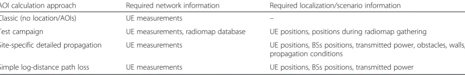
Different approaches can be adopted to define the AOIs by approximating Eq. (4) for any given (x,y,z). Particu-larly,test campaigns,site-specific detailed-scenario propa-gation models (considering specific obstacles, walls, etc.) or simplelog-distance path loss(assuming all points as in

line-of sight to the BSs) can be adopted. The applica-tion of one or another technique for the AOI calculaapplica-tion is dependent on the available information about the scenario.

Table 1 summarizes the information required for the location-based indicators depending on the approach used for the AOIs estimation. Here, the transmitted cell power can be obtained from the normal configuration/ monitoring of the BSs. However, the availability of the rest of the information has to be analyzed.

On the one hand, in common situations, test campaigns or detailed-scenario models (including obstacles, walls, etc.) are not available, making not possible to apply detailed-sce-nario propagation models for AOI estimation. Add-itionally, the details of such information can become rapidly obsolete if the scenario changes.

On the other hand,simplelog-distance path loss calcu-lation (not considering site-specific walls and obstacles) only requires the positions and relative power of the base stations (BSs). The knowledge about the BSs positions might be not available if the deployment isunplanned, as it can be especially the casehome femtocells. However, the BSs position is typically known for the type of large indoor scenarios (malls, large office, airports) considered. In these environments, BSs (picocells or enterprise femtocells) are mainly installed in fixed positions by professional field en-gineers, allowing the registry of their locations. For these scenarios, careful planning of the deployment is also recommended [24]. Additionally, if the cellular network supports UE positioning, the location of the BSs will be also required for such service.

Although not considering site-specific details can led to inaccuracies, it has to be noted that this assumption is only used to estimate geographical AOIs, not to obtain detailed RSS values. Also, many indoor large scenarios are semi-unobstructed or containing symmetric obstacles (e.g., walls) for the different BSs, minimizing also the importance of a very detailed propagation approach to calculate the AOIs.

Therefore, taking into account the issues associated with more complex approaches (particularly the lack of the necessary information), simple log-distance path loss would commonly be the most feasible solution to estimate the AOIs in many real deployments scenarios. In this case, for the AOIs definition, a similar reasoning to the one followed in [25] for coverage probability estimation is adopted. For each point (x,y,z), the expected received power from celli, value RSS^ ððx;y;zÞ;celliÞ, consists of

the transmitted power of the cell, Ptx(celli) minus the path loss to that point PL((x,y,z), celli). Without in-cluding fading effects, the path loss is inversely propor-tional to the distance between the point and the cell:

^

RSSððx;y;zÞ;celliÞe10 logðPtxðcelliÞ=d∝ððx;y;zÞ;celliÞÞ

path loss exponent. This exponent has commonly a value close to 2 for line-of-sight propagation in indoor environments (e.g., ∝= 1.87 for Winner II indoor-indoor A1 model [26]).

Fast-fading effects in the propagation are not included. This is consistent with their reduced values in the final coverage due to the terminal interleaver and the existent time and power margins for mobility and cell reselection.

If, as expected, the obstacles of the scenario are un-known and the cells transmit roughly in the same band (as it is typically the case), the expression of ECov based on Eq. (4) should be approximated as:

ECov cellð iÞ ¼ ðx;yÞ∈E2

This expression is equivalent to a multiplicatively weighted Voronoi tessellation [25]. If all the small cells transmit with the same power, this is equivalent to the classic polygonal Voronoi tessellation:

However, if the BSs transmitted powers are not equal, coverage areas might be non-convex, non-polygonal and they can include “holes”. This highly increases the com-plexity of calculating whether a point belongs or not to the

AOI. To avoid these issues, the work in [25] proposed a circular approximation to the coverage:

RcovðcelliÞ ¼ _∀min_i≠j

Following the same approach, ECent(celli) can be cal-culated as a circle centered in the BS with a radius equivalent to a configurable portion, kR∈[0, 1], of the minimum distance between the BS and the border of its coverage: Rcent(celli) =kR*Rcov(celli). In this way, the marginΔRSScentas defined in Eq. (4) would be

equiva-lent to:

These expressions allow to compute the AOIs prior to the online detection, storing them with a very reduced cost, whereas they also allow direct AOI reconfiguration if there are changes in the transmitted power.

For the sample weights, an increasing relevance should be given to those positions better covered by celli and less covered by its neighbors in normal operation. As-suming also a simple approach for their definition, the proposed expression for the weight is:

wcelli

where celldom is the dominant adjacent cell which highest

estimated received power on (x,y), celldom: {Ptx(celldom)/

d((x,y), celldom)∝>Ptx(cellj)/d((x,y), cellj)∝|∀j≠i,∀j≠dom}. In this way, and with ECov and ECent following the same propagation approach, the computation of wcelli

AOI γxyz

consists in a simple point-in-polygon (PIP) [27] and/or point-in-circle calculation.

4 Detection algorithm

Based on any available indicatorF, typical detection mech-anisms are based on calculating which of its samples crosses a predefined detection threshold, considering then that the network is under failure [28]. The presented indi-cators (RSS_meanorRSS_5th percentile, location-based or not) could be straightforwardly used for this process.

This detection approach has important advantages in comparison with more complex mechanisms, like the ones presented in reference [6], as it allows the immediate de-tection of degradations based on a unique indicator and in a fast manner. However, it implies the definition of thresh-olds, typically by human expertise, being each considered indicator associated with a particular threshold. Threshold definition is commonly a costly task that implies large

Table 1Required information depending on the AOI calculation approach

AOI calculation approach Required network information Required localization/scenario information

Classic (no location/AOIs) UE measurements –

Test campaign UE measurements, radiomap database UE positions, positions during radiomap gathering

Site-specific detailed propagation UE measurements UE positions, BSs positions, transmitted power, obstacles, walls, propagation conditions

times and a deep knowledge of the network behavior that may be not available. Additionally, the thresholds may vary depending on the specific network or BS, complicating their definition.

To avoid this issue, a baseline method based on a naive Bayes classifier is proposed. For its description, up-percase letters will refer to variables/indicators, lowercase to specific values of such variables and bold letters to vec-tors of multiple variables or values. The Bayes classifier method would make use of any set of input indicators

F= {F1,F2,…} and their current values, e.g., f[t] = {F1= f1[t],F2=f2[t],…} in order to estimate the posterior probability p C^ð i¼cijF ¼f½ tÞ of a celli of being in a certaincell status Ci=ci, whereci∈{Normali, Sleepingi}. This process is based on two main stages: a training phaseand an online phasethat should be performed (in parallel) for any celliconsidered for analysis.

4.1 Training phase

During this initial stage, the conditional probability density functions(PDF) of allF∈Findicators given both normal and failure case has to be estimated: ^p Fð j

NormaliÞ and ^p Fð jSleepingiÞ, as well as the prior

prob-abilities,p^ðNormaliÞ, andp^ Sleepingi

of the cell status. The PDFs are calculated from the relative frequency of the values in the training set. Then, the kernel smoothing (KS) density approximation [29] is proposed for estimat-ing the PDFs. KS probabilistic model is generated based on the superposition of multiple Gaussian functions. Con-versely, it is commonly assumed that RSS-based indicators values can be modeled by a unique Gaussian or Beta dis-tributions. However, this assumption is only correct for uniform users’distributions and non-limited areas of ana-lysis. As it would be shown in the evaluation section, this is not the case for data obtained in more irregular scenar-ios with complex user mobility. The KS solution is non-parametric and more computationally expensive than other mechanisms. However, this problem can be miti-gated for real-time detection as the model is fitted during the training phase, and it is already constructed in the on-line phase. To save storage space, the KS distribution is calculated only in the range of discrete RSS values that can be reported by the UE, which depends on the particu-lar standard.

Therefore, the stored conditional PDF for each pos-sible statusCi(normal or sleeping) is a discrete function such as pdfFð Þ ¼rF fp r^ðFj ÞCi j∀rFRG pdfð FÞg, whererF is any of the discrete values of the range RG(pdfF(rF)) where the distribution is defined. For example, in LTE and considering RSRP values, RG(pdfF) is equal to the set of integers in the interval [0…97], which is a direct mapping of the receive power measurements from−140 to−44 dBm with a 1-dB resolution [20].

However, during the online phase, the mean or per-centile obtained from the set of multiple of RSS samples can result in values not included in RG(pdfF). In that case, KS smoothing or simpler linear approximation be-tween the immediately lower and higher integer values can be applied depending on the available computational capacity.

One issue for this approach would be obtaining the values for the training set. For the normal status, this is easy to obtain, as the indicator values can be gathered under the normal behavior of the network. For the sleep-ing cell status, if real fault-labeled cases are not available (which is the most common situation), two different options are envisaged:

ON/OFF calibration period: by a simple procedure of disconnecting and connecting the cells in an alternative manner (which can be performed automatically), the system can obtain the needed sleeping cell training set. These may however alter the normal operation of the network.

Neighboring cells measurements analysis: if the terminals are able to measure and report RSS values from neighboring cells, this information can be used to approximate their expected serving cell values if one cell is disconnected. This process would have the advantage of not disrupting the cell service provision, and it could be performed continuously.

Independently, of the used method, the validity of the calculated models can be jeopardized by changes in the network: in the BSs positions, in the scenario characteris-tics, obstacles, etc. In such cases, mechanisms for automatic update of the models shall be applied. Here, reference [30] provided a solution for identifying the need of updating the models as well as online updating. Such mechanisms can be straightforwardly applied to any network indicator, not requiring therefore any particular modification for the proposed location-based approach.

4.2 Online phase

This stage is performed in the already working network. Here, the estimated status of celli is calculated by a pro-posed feature-weighted version of the naive Bayes classifier. The followed concept of weighted naive Bayes classifier was proposed in [31] for general centralized data mining. In the present work, however, the applied weights, expres-sions, and application have been completely redefined for its use in cellular distributed failure detection.

In this way, the Bayes classifier is used to combine the values off[t]. For anyCi=ciof the two possible sta-tus of celli,Ci= {Normali, Sleepingi}, ^p Cð i¼cijF ¼f½ tÞ

^

status value; this means, the total likelihood of the status if no data is known. p^ðF ¼f½ tÞ is the estimated likeli-hood of the evidence. ^p Fð ¼f t½ jCi¼ciÞ is the

condi-tional probability for a particular input indicator value F=f[t] given the status ci of celli and calculated as de-scribed from the pdfF(rF).ΩF[t] is the confidence levelof thef[t] value, and it is used to modulate the contribution of each value of FAOI_ij in the weighted classifier in each instant.

The consideration of independence between the vari-ables in F is disputable; however, it is commonly as-sumed for cellular indicators [11]. Also, naive Bayes classifiers have demonstrated good results even when that condition is not fulfilled [32]. Based on this, the es-timated status of celli,ĉiis obtained by choosing the sta-tus with the highest posterior probability. As only two possible statuses have been defined Ci= {Normali, Slee-pingi} and being the evidence equal to both, the classifier expression can be simplified to:

^ portance of each indicator in the classification. To do so, a particular definition of this parameter is established, defined as a function of thenumber of samples used for the calculation off[t] (|MF[t]|), theweight relevance factor (φF[t]) of those measurements (ifFis a location-based in-dicator), as well as thestatistical difference(Ψ(F)) between

Fnormal and sleeping PDFs.

Firstly, |MF[t]| is used to define a minimum number of samples, |M|th, to consider the indicator significant. Secondly, in the case whereFis a location-based indica-tor, φF[t] is calculated by the normalized sum of the sample weights applied to the RSS measurements, giving higher weight to those f[t] based on larger number of samples and/or more relevant ones:

φF½ ¼t

where φ_F½ t represents the normalization factor, being the average of the relevant factors applied intto all the indicators inF.

Thirdly, Ψ(F) is calculated following the Hellinger score [33], serving as a metric of the level of overlapping between the normal and sleeping PDFs of F. This is where it is applied to the discrete conditional PDFs:

Ψ FAOI_ij

In comparison to other statistical distances (like the Kullback–Leibler divergence proposed in [31]), the Hel-linger metric has the advantages of being symmetric (H(P,Q) =H(Q,P) for anyQ,Pdistributions) and satisfying the expression 0≤H≤1, where “0” indicates complete similarity while “1” means complete independency, be-ing a parameter of easy incorporation to any decision algorithm.

With these three parameters, the expression of ΩF[t] is finally defined as:

ΩF½ ¼t jMF½ tj<j jMth

φF½ t Ψð ÞF ð14Þ

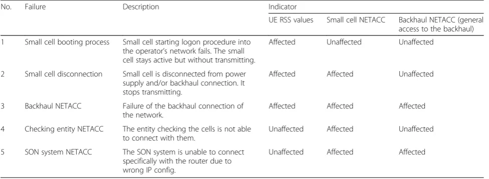
5 Diagnosis of sleeping cell causes

Once the sleeping cell problem is detected, compensation and recovery mechanisms can be supported by knowledge on the root cause behind the problem. In that respect, Table 2 shows the main causes of failures in small cell net-works. Here, causes 1, 2, and 3 represent the most com-mon roots for the catatonic sleeping cell problem in small cell networks. Four and 5 are failures in the OAM system that could lead to the erroneous identification of the cell issue in classic approaches.

While the presented detection mechanism has been centered on UE RSS analysis, other inputs can be used for the assessment of cellular degradations. These come from the analysis of the network accessibility(NETACC) of the cellular system elements from the point of view of their non-cellular links: LAN, optical fiber, DSL, etc. This can be checked by centralized SON entities as well as between small cells. An element in charge of that task is named as NETACC checking entity. This element or elements can perform the checking periodically or follow-ing an event/demand [9]. This check can be performed for a specific small cell element or for the complete deploy-ment backhaul, e.g., by IP-PING style messages. Such in-formation can be modeled as a binary random variable whose value is“1”if the element analyzed is reachable and

“0”otherwise.

simple rules are proposed for the diagnosis of the differ-ent cases, as shown in Table 2.

6 Distributed Self-healing scheme

The implementation of SON mechanisms in current heterogeneous networks brings several issues to the classic centralized approach for OAM in cellular systems. Firstly, one of the main challenges to achieve fast-response failure management in cellular networks is the associated delay and signaling cost of the communications between the central OAM systems and the network elements (UEs, BSs). The network backhaul can be easily overloaded by the signaling costs associated with network monitoring. This is especially the case for femtocells, which make use of non-dedicated consumer-oriented infrastructure. Secondly, the growing number of cells and the complexity of the network might even lead to saturation of the operator’s backbone and central OAM elements, as they are in charge of monitoring and operating huge number of network elements.

In order to avoid these issues, the elements of each de-ployment should be able to manage themselves. Thus, a distributed scheme is deemed indispensable for the proper performance of the network. In this field, previous work [9] aimed to reduce signaling costs in femtocell deployments by establishing a local OAM element, allowing hybrid algo-rithms and minimizing backhaul use. Additionally, since the proposed on-site OAM element was only responsible for a local small cell network, the number of cells to be op-erated by such entity is much reduced, significantly limiting computational costs. While such scheme could be adopted for the mechanisms proposed in the present work, it is still vulnerable to failure in that centralized entity. Also the small cells may not be part of the same LAN, or their interconnection capacity may be low (e.g., if it is based on WiFi-LAN). Conversely, the use of a fully distributed algo-rithm would increase the resiliency of the system.

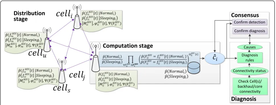
6.1 Distributed scheme

Given the presented detection and diagnosis mechanisms, a procedure is defined for its distributed application. The proposed approach is based on the collaborative classifica-tion of any celli status,Ci by itself and its neighbor cells. This implies that, for the analysis of possible failures in celli, each cellj∈cellsimpi would be involved in the process,

where cellsimp_i is the set of sites that would be impacted by the possible failure: typically, celliitself and its adjacent ones (as graphically represented in Fig. 1).

The simplified detection rule presented in Eq. (11) has as input a set of indicators calculated from the cellsimp_i . In this scheme, each cellj is in charge of computing an indicator FAOI_ij ∈FAOI_i . This is calculated from the mea-surements MAOI

ij ½ t , consisting on those measurements

served by cellj in a certain AOI (e.g., ECov or ECent) of celli. For example, the RSS_5th percentile of the UEs served by the celljin ECov(celli). In this way, the samples are lo-cally gathered and aggregated, minimizing signaling costs.

The complete self-healing distributed procedure is pre-sented from the perspective of any cellj participating in the detection of a possible faulty celli. cellj will apply the same process for any cellisuch that cellj∈cellsimp_i . In the

description of the different phases, the expressions and variables already described would be particularized for the distributed case:

1. Definition of cellsimp_i and AOIs

In order to define the cells likely to be affected by a failure in a particular celli, the approach is to

automatically include incellsim_i pthe celliitself and

its adjacent neighbors. The adjacent cells can be defined from the estimated coverage area maps, selecting the BSs whose coverage areas are in contact.cellsimp_i set can also be updated based on

Table 2Sleeping small cell causes and reachability

No. Failure Description Indicator

UE RSS values Small cell NETACC Backhaul NETACC (general access to the backhaul)

1 Small cell booting process Small cell starting logon procedure into the operator’s network fails. The small cell stays active but without transmitting.

Affected Unaffected Unaffected

2 Small cell disconnection Small cell is disconnected from power supply and/or backhaul connection. It stops transmitting.

Affected Affected Unaffected

3 Backhaul NETACC Failure of the backhaul connection of the network.

Affected Affected Affected

4 Checking entity NETACC The entity checking the cells is not able to connect with them.

Unaffected Affected Unaffected

5 SON system NETACC The SON system is unable to connect specifically with the router due to wrong IP config.

the neighbor cell list of each cell, as they are automatically updated during network operation [31]. All the cells in the deployment should have knowledge of the differentcellsimp_i sets and their relative position in order to participate in the detection of problems of those sets where they are part of.

Based oncellsimp_i and their relative positions, the AOIs of cellican be calculated (in a centralized or

distributed way) and stored.

2. Training phase

As described in Section4, celljparticipating in the

detection of a failure in cellineeds to be in

possession of the prior likelihood of each status and the conditional PDFs: pdfAOI;Normali

ij rij and p

dfAOI; Sleepingi

ij rij (where its previously presented

nomenclature has been particularized for the indicatorFAOI_ij ). During the training phase, the PDFs can be constructed and stored directly by celljas

FAOI_ij is locally generated by the BS. From these, theΨ FAOI_ij

parameter can be also calculated and stored. The prior likelihoods are assigned with a default or configured value.

3. Online phase

During the operational life of the network, the process is divided in different stages of

computation and information sharing between the cells.

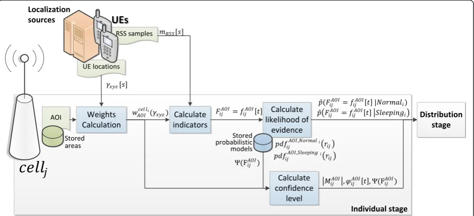
3.a Individual stage

This stage is described in Fig.2. Firstly, cellj

gathers the RSS samples reported by its served UEs. Secondly, the localization associated with each

measurement is obtained directly from localization sources that can be the UEs themselves, a cellular-based positioning system or an external localization service [9]. Thirdly, with this information and the stored AOIs, the values of thewcelli

AOIare calculated

for all the RSS samples and then the location-based indicator valueFAOI_ij ¼fAOI_ij ½ t is obtained.

Fourthly, based on this and the conditional PDFs, the likelihoods of the current value given the status of celli,p F^ AOIij ¼fAOIij ½ t jNormalÞ

and^p FAOI_ij ¼fAOI_ij ½ t jSleepingÞ

are calculated as well asφAOI

ij ½ t (see Eq. (13)). Also, the number of samples inside the AOI and used to generate the indicator are propagated to the following distribution stage.

3.b Distribution stage

Afterwards, each cell of cellsimp_i shares their estimated conditional probabilities with the rest of the cells of the set. This and the next stages are presented in Fig.3.

The message from a cell might be not received due to incorrect timing, connection losses, or failure in the cell, which cannot be considered a univocal consequence of a sleeping cell failure (as described in Section5). Therefore, the conditional probabilities for the indicator of that cell are assumed“1”for both status, which means that such input is not considered in the classifier.

3.c Computation stage

Having the conditional probabilities from the other cells of cellsimp_i , the status of cellican be

calculated by any of them based on the naive Bayes classifier detection rule presented in Eq. (15), providing its estimated status.

3.d Diagnosis stage

If a neighboring cell is detected as sleeping, any other BS can check its NETACC in order to determine the particular cause behind the problem. This, together with the estimated status is used to specify the particular cause by means of binary logic following Table2.

3.e Consensus

If the information has been properly received and computed by each BS, the results in terms of the estimated status shall be equivalent to all of them. However, this may not be the case if any

distributed message is lost. Also, if the NETACC check provides different results (e.g., due to congestion) for different BSs.

Therefore,consensustechniques can be applied for the results achieved by all of the BSs. In order to achieve a common diagnosis from the possible different results of each node, multiple mechanisms have been developed for the general field of

distributed computation. For example, the selection of a master/coordinator cell dedicated to perform the final posterior probability calculations and then share them with the other cells can keep consensus as well as reduce the computational costs by freeing some of the BSs from the need of performing the classification [31]. However, the system becomes then more vulnerable to failures in such master cell. To avoid so, the use of strong consistency as presented in [34] is recommended. This is based on making the independent diagnosis performed by each cell consistent by sharing and checking their mutual results.

4. Compensation/recovery activity

Once the cell status is detected and diagnosed, compensation and recovery mechanisms can be triggered. For instance, readjusting cell powers to compensate a neighboring sleeping cell, rebooting automatically themselves if found faulty or alert the operator’s OAM system about the issue.

6.2 Implementation

The proposed distributed system would benefit for the direct interconnection of the cells, preferably by local high performance connections such as Ethernet LAN. That is the case for femtocell deployments, where the cells are often connected to the same router and/or access point to the Internet backhaul. There, local IP access (LIPA) [35] protocols can be used for over-the-top imple-mentations of the proposed distributed approach. In a more standardized manner, the proposed communications can be integrated through the LTE/LTE-A defined X2 interface between the cells.

The distribution phase could also make use of multicast-type protocols, where the deployed cells can be grouped to reduce the need of addressing the messages to particular base stations.

Moreover, the proposed approach requires a level of synchronization between the cells in order to share the same monitoring and message exchange periods. Such synchronization is already present as part of the coord-ination between the cellular network elements, and the proposed system does not introduce any additional requirement.

7 Evaluation

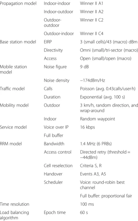
For the evaluation of the proposed mechanisms, the system level simulator detailed in [36] was extended to integrate the proposed mechanisms as well as cell

faults. The defined simulation parameters are included in Table 3. As baseline RAT, LTE is chosen. The radio environment is simulated by Winner II propagation model [26], where fast-fading is modeled by the Ex-tended Indoor A model [37]. RSS-type information is provided by the LTE RSRP metric. The simulated sce-nario follows an expected typical 5G deployment com-prising 12 small cells with a reduced average inter-site distance of 50 meters. Fully variable user distributions are emulated in a realistic airport model: Málaga air-port, IATA code: AGP (ranked the 33rd busiest airport in Europe with 12.5 million passengers per year) is se-lected as a key scenario for the deployment (see Fig. 4). This indoor location is placed in a large external area (3 × 2.6 km2), where a macrocell station is located at 500 m from the airport.

In the simulation, it is assumed that UEs report RSRP values and locations once per second. This is consistent with the signaling constraints of possible over-the-top implementations [9], whereas control plane solutions

may allow higher frequency reporting (as 0.1 s considered in [12]).

Catatonic sleeping cells are modeled in the simulation in the following way: for each possible faulty cell 400 continuous monitoring periods of 1 m are simulated: first 200 periods corresponding to a normal case situation (where the cell works properly), while the following 200 periods model a sleeping cell failure of one BS that stops transmitting. During these periods, the movement of users along the airport is modeled based on random waypoint including realistic users’concentration in security check-points and boarding gates areas.

7.1 Impact of sleeping cell case in classic performance indicators

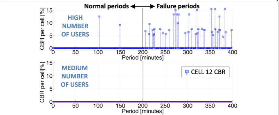
For the presented set-up, Fig. 5 shows the call blocking ratio (CBR); this means, the percentage of calls not able to access the cellular network. CBR is commonly used as an indicator of network accessibility and applied on the analysis of possible network failures. The figure reflects the common case where a sleeping cell failure (in this case, cell 11) cannot be spotted by purely classical performance indicators.

On the one hand, Fig. 5, top, presents a situation with a high number of average users per cell (around 12 active users simultaneously). In this case, the CBR of the neigh-boring cell 12 highly increases after the failure of cell 11. However, it is observed that there are some peaks of high CBR even in normal status, as well as quite few periods with low CBR under failure condition.

On the other hand, Fig. 5, bottom, presents a situation with a reduced number of users (an average of 7 UEs per cell). For this case, the CBR is not impacted at all by the failure, making impossible its detection based on this metric.

7.2 RSS indicators and AOIs

Hereafter, the indicators proposed for the RSS-based detection are assessed with different restrictions in terms of the area selected and the distributed/centralized approach, particularized for the case where cell 11 is faulty (cellsimp₁₁ ¼f9;10;11;12g).

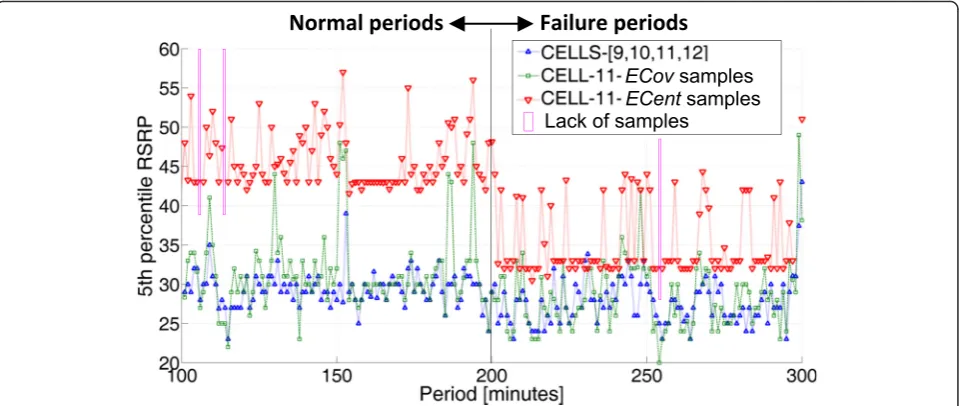
Figure 6 compares the classic RSS 5th percentile values for the UE served by the cells in cellsimp₁₁ with the ones obtained applying ECov and ECent (withkR= 0.75) calculated following the simple log-distance propagation approach and the sample weights defined in Eq. (9) for any serving cell. The results for both ECov and ECent are assessed and compared as alternative AOI defini-tions, where ECent represents a far more restricted area than ECov.

It can be seen how the classic indicator do not show any clear impact due to the failure in most of the loops.

Table 3Simulation parameters

Propagation model Indoor-indoor Winner II A1

Indoor-outdoor Winner II A2

Outdoor-outdoor

Winner II C2

Outdoor-indoor Winner II C4

Base station model EIRP 3 (small cells)/43 (macro) dBm

Directivity Omni (small)/tri-sector (macro)

Access Open (small)/open (macro)

Mobile station model

Noise figure 9 dB

Noise density −174dBm/Hz

Traffic model Calls Poisson (avg. 0.43calls/user·h)

Duration Exponential (avg. 100 s)

Mobility model Outdoor 3 km/h, random direction, and wrap-around

Indoor Random waypoint

Service model Voice over IP 16 kbps

Full buffer

RRM model Bandwidth 1.4 MHz (6 PRBs)

Access control Directed retry (threshold = −44dBm)

Cell reselection Criteria S, R

Handover Events A3, A5

Scheduler Voice: round-robin best channel

Full buffer: proportional fair

Time resolution 100 ms

Load balancing algorithm

However, the variation is evident for the ones using loca-tion ECent thanks to the selecloca-tion of the most relevant samples and their weighting. Also it could be observed how some periods (e.g., 106, 114, and 254) have no values for the ECent indicator due to the lack of UEs in the area. This indicates how reducing the AOI increases the visibility of the failure impact but also increments the possibility of not having enough samples to generate the metric.

7.2.1 Detection performance

The proposed detection Bayes scheme is applied for lo-cation and non-lolo-cation indicators as well as centralized (not filtering the RSS measurements by serving cell) and distributed approaches. In the evaluation, the training

phase is performed using as calibration set 50 periods under each cell status, where these periods are considered as previously labeled. As commented, in real deployments the training set can be obtained from real failure recorded cases, by an operator defined ON/OFF calibration phase or from neighboring cells measurements analysis as indi-cated in Section 4.A. The conditional PDFs are therefore obtained from this training set. A value of |M|th= 10 is

also established. RSS 5th percentile statistics are selected as inputs for the classifier, as they show a higher variation between the normal and sleeping cases than the indicators based on the RSS mean.

Common figures of merit for detection are the false normalrate (FN), being the ratio of faulty periods identi-fied as normal; false alarm rate (FA), the percentage of

Fig. 4Evaluation scenario

normal periods identified as faulty; and the inconclusive

rate (IN), or the percentage of periods where there is no UE RSS measurements in the considered AOI and no detection is performed.

Figure 7 shows the FA, FN, and IN values for the dif-ferent combinations of detection options and for the case where cell 11 is analyzed.Non-location local refers to the classic detection performed based uniquely on the 5th percentile of the UE served by the most affected neighbor (cell 12 in this case). Non-location centralized

refers to the classic approach of using the 5th percentile of the RSRP values gathered by all UEs served by cellsimp₁₁ .

Non-location distributedfollows the proposed distribution algorithm but applied over-the-classic RSRP indicators from the UE served by each cell. Centralized ECov and ECent make use of the proposed location-based approach generating the indicators based on the samples gathered in the AOIs without distinguishing their serving cell. Fi-nally, distributed ECov and ECent follows the complete

proposed location-based distributed approach presented in Section 6.

For non-location-based approaches, it can be observed how the use of the distributed approach highly increases the accuracy of the detection, achieving FA = 0 % with respect to the centralized and local approaches. How-ever, the similarity between the classic RSRP values for both normal a faulty status causes a high FN = 21 %. The use of localization highly improves this aspect: while the use of ECov does not introduce significant improvement in the detection due to its wide area, ECent achieves FN = 1 %, highly outperforming previ-ous approaches.

The study is extended to the rest of the central cells of the scenario {9, 10, 11, 12}, where the failure of each of them is modeled. The resultant detection performances in percentage are shown in Table 4. It is observed how the results of the distributed location-based proposed approach highly outperformed those of the classic

Fig. 6Location-based fifth percentile RSRP indicators for different AOIs

mechanisms except for the cell 12 case. This low per-formance is due to the complex wall environment sur-rounding such station, which makes that even in normal operation, cell 11 serves a high amount of users in the ECent of cell 12. This indicates how more complex defi-nitions of the AOIs (such as those based on the de-scribed detailed propagation models) might be required where these situations are present in the deployment.

For the rest of the cells, the distributed approaches highly improve the results of their equivalent centralized or local methods. Moreover, the use of location-based indicators provides far better performance than classic ones. Also, the use of the narrower ECent instead of ECov allows reduced FA and FN at the cost of increasing IN, due to the minor number of available measurements in the AOI.

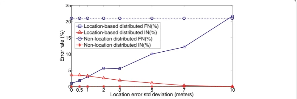
7.3 Impact of UE localization error

The previous evaluation demonstrates the capabilities of the location-based approach to improve sleeping cell de-tection mechanisms. However, one of the main charac-teristics to take into account for its applicability is its robustness to localization inaccuracies. These are mod-eled in the simulator by an added Zero-mean Gaussian noise to the real location of each terminal before feeding

the self-healing algorithms with this data, following the expression:

where eux and euy are the added error distance for each coordinate, and μ and σ are respectively the mean and deviation of the normal distribution Ɲ, being consistent to the most common approach for error modeling of positioning methods [38]. In this way, the system is tested for different values of the location error standard deviation σ= {0, 0.5, 1, 2, 3, 5, 7, 10}, which is equiva-lent to the root mean squared position error (RMSE) of the positioning technique. Such error levels cover from very precise indoor positioning solutions as UWB-based (e.g., reference [15] proposed technique achieves around 1-m mean accuracy in real experiments) to just an extremely rough estimation, including more common positioning mechanisms as WiFi-based (e.g., the system developed in [14] showed mean errors of 7 m in real scenarios).

The average results for cell 11 given those errors are presented in Fig. 8 for the ECent distributed non-location and non-location-based techniques. FA is not

Table 4Summary of detection performance for different cells

Cell Cell 9 Cell 10 Cell 11 Cell 12

Indicator type\figure of merit FN FA IN FN FA IN FN FA IN FN FA IN

Non-location local 69.0 25.6 0.0 13.5 35.2 0.0 17.5 44.7 0.0 39.5 19.1 0.0

Non-location centralised 46.0 45.7 0.0 19.0 29.1 0.0 33.5 28.1 0.0 48.5 9.5 0.0

Non-location distributed 22.0 0.0 0.0 14.0 0.0 0.0 21.0 0.0 0.0 35.0 0.0 0.0

Centralised ECov 13.0 15.1 10.5 3.5 0.5 2.8 31.5 37.7 0.0 35.0 21.1 0.0

Centralised ECent 7.0 0.0 40.1 2.5 0.5 17.8 21.5 0.5 3.3 63.5 0.0 4.3

Distributed Ecov 3.5 0.5 10.8 0.0 0.0 2.8 21.5 0.0 0.0 57.0 0.0 0.8

Distributed Ecent 0.0 0.0 40.6 0.0 0.0 18.0 1.0 0.0 3.5 53.5 0.0 5.0

included in the graph as it is always 0. The figure shows the robustness of the location-based approach even for large inaccuracies, keeping a much better performance than non-location ones even for very high-positioning errors as 7 m.

8 Conclusions

This work has assessed the use of classic network indica-tors for sleeping cell failure detection in dense networks, showing the reduced impact that they might reflect. This would commonly lead to delay or wrong detection of network issues based on those indicators.

To overcome this issue, the use of location-supported metrics has been proposed. Such metrics highly increase the capability to detect cell failures. In this way, the pro-posed location-based indicators support the design of troubleshooting systems with improved failure detection than previous schemes. These have been integrated in a newly defined cell distributed detection and diagnosis al-gorithm, where the required associated architecture and methodology have been defined.

The proposed system has been assessed with a system level simulator that models a representative DenseNet indoor scenario. The evaluation has shown how the pro-posed approach highly outperforms the results achieved by classic mechanisms and by centralized implementa-tions. The behavior of the algorithm in the presence of inaccuracies in the localization information has also been analyzed, showing high robustness for the normal levels of inaccuracies found in existing positioning systems.

Future works will analyze the extension of the pro-posed approach to scenarios including additional hetero-geneity, combining different cellular and non-cellular systems. Also, the impact of additional 5G radio conditions, such as higher frequency radio links, will be further explored.

Abbreviations

3GPP, Third Generation Partnership Project; CBR, call blocking ratio; CQI, channel quality indicator; DenseNet, Dense Network; ECent, expected center area; ECov, expected coverage area; EIRP, equivalent isotropically radiated power; FA, false alarm rate; FN, false normal rate; IATA, International Air Transport Association; IN, inconclusive rate; KPI, key performance indicators; LTE, long-term evolution; NGMN, next-generation mobile networks; PDF, probability density function; PRB, physical resource block; RAT, radio access technology; RFID, radio-frequency identification; RRM, radio resource management; RSRP, reference signal received power; SINR, signal to interference-plus-noise; SON, self-organizing networks; UE, user equipment; UWB, ultra-wideBand; VoIP, voice over IP

Competing interests

The authors declare that they have no competing interests.

Acknowledgements

This work has been funded by Junta de Andalucía (Proyecto de

Investigación de Excelencia P12-TIC-2905), and Spanish Ministry of Economy and Competitiveness / FEDER (TEC2015-69982-R and Network of Excellence Red ARCO 5G, TEC2014-56469-REDT).

Received: 1 August 2015 Accepted: 23 June 2016

References

1. “What is 5G? 5G visions”. GSM history: history of GSM, mobile networks, vintage mobiles. Online: http://www.gsmhistory.com/5g/. Accessed 14 June 2016 2. D Lopez-Perez, M Ding, H Claussen, AH Jafari, Towards 1 Gbps/UE in

Cellular Systems: Understanding Ultra-Dense Small Cell Deployments. IEEE Commun. Surv. Tutorials17(4):2078–2101 (2015). doi:10.1109/COMST.2015. 2439636

3. “Small cells—what’s the big idea? Femtocells are expanding beyond the home,” White Paper, Small Cell Forum, 2012. http://smallcellforum.org/smallcellforum/ Files/File/SCF-Small_Cells_White_Paper.pdf

4. 3GPP, Telecommunication management; principles and high level requirements, TS 32.101, 3rd Generation Partnership Project (3GPP) (2015). http://www.3gpp. org/ftp/Specs/html-info/32101.htm

5. 3GPP,“Telecommunication management; self-organizing networks (SON); self-healing concepts and requirements,_”3rd Generation Partnership Project (3GPP), TS 32.541, 2016. http://www.3gpp.org/DynaReport/32541.htm 6. F Chernogorov, T Ristaniemi, K Brigatti, S Chernov,“N-gram analysis for

sleeping cell detection in LTE networks,”2013 IEEE International Conference on Acoustics, Speech and Signal Processing, Vancouver, BC. 2013, pp. 4439_– 4443. doi: 10.1109/ICASSP.2013.6638499

7. T Perry,The Indoor Navigation Battle Heats Up IEEE Spectrum magazine, (IEEE, New York, US, 2012). http://spectrum.ieee.org/tech-talk/consumer-electronics/portable-devices/the-indoornavigation-battle-heats-up 8. M Molina-García, J Calle-Sánchez, JI Alonso, A Fernández-Durán, FB Barba,

Enhanced in-building fingerprint positioning using femtocell networks. Bell Labs Tech. J.18(2), 195–211 (2013)

9. S Fortes, A Aguilar-García, R Barco, F Barba, J luque, A Fernández-Durán, Management architecture for location-aware self-organizing LTE/LTE-a small cell networks. IEEE Commun. Mag.53(1), 294–302 (2015)

10. A Aguilar-Garcia, S Fortes, M Molina-García, J Calle-Sánchez, JI Alonso, A Garrido, A Fernández-Durán, R Barco, Location-aware self-organizing methods in femtocell networks. Comput. Netw.93(1), 125–140 (2015) 11. R Barco, P Lazaro, P Munoz, A unified framework for self-healing in wireless

networks. IEEE Commun. Mag.50(12), 134–142 (2012)

12. W Wei, L Qing, Z Qian, COD: a cooperative cell outage detection architecture for self-organizing femtocell networks. IEEE Trans. Wirel. Commun.

13(11), 6007–6014 (2014)

13. K Bouchard, D Fortin-Simard, S Gaboury, B Bouchard, A Bouzouane, Accurate trilateration for passive RFID localization in smart homes. Int. J. Wireless Inf. Networks21, 32–47 (2014)

14. M Raitoharju, H Nurminen, R Piché, Kalman filter with a linear state model for PDR+WLAN positioning and its application to assisting a particle filter. EURASIP J. Adv. Signal Process. 2015, 1_–13 (2015). doi:10.1186/s13634-015-0216-z

15. P Muller, H Wymeersch, R Piche, UWB positioning with generalized gaussian mixture filters. IEEE Trans. Mob. Comput.13(10), 2406–2414 (2014). doi:10.1109/TMC.2014.2307301

16. G-NetTrack phone measurement capabilities. [Online]. Available: http:// www.gyokovsolutions.com/survey/surveyresults.php. Accessed 14 June 2016 17. S Fortes, AA Garcia, JA Fernandez-Luque et al., Context-aware self-healing:

user equipment as the main source of information for small-cell indoor networks. IEEE Veh Technol Mag11, 76–85 (2016). doi:10.1109/MVT.2015. 2479657

18. ERICSSON,“App Experience Optimization,”Webpage. [Online]. Available: http://www.ericsson.com/ourportfolio/services/app-experience-optimization?nav=fgb_101_108|fgb_101_592. Accessed 14 June 2016 19. 3GPP,“Universal Mobile Telecommunications System (UMTS); Physical layer;

Measurements (TDD),”3rd Generation Partnership Project (3GPP), TS 25.225, 2015. http://www.3gpp.org/DynaReport/25215.htm

20. 3GPP,“LTE; Evolved Universal Terrestrial Radio Access (E-UTRA); Requirements for Support of Radio Resource Management,”3rd Generation Partnership Project (3GPP), TS 36.133, 2014.

21. R Groves, F Fowler, M Couper, J Lepkowski, E Singer, R Tourangeau,Survey Methodology, ser. Wiley Series in Survey Methodology (Wiley, United States, 2009).

23. E Langford, Quartiles in elementary statistics. J. Stat. Educ.14, 3 (2006) 24. Small Cell Forum,Enterprise femtocell deployment guidelines, 2013 25. B Tianyang, RW Heath, Location-specific coverage in heterogeneous networks.

IEEE Signal Process Lett.20(9), 873–876 (2013)

26. WINNER II IST project,“D1.1.2. WINNER II channel models. part II. radio channel measurement and analysis results. v1.0,_”WINNER II IST project, Tech. Rep., 2007. [Online]. Available: www.ist-winner.org/. Accessed 14 June 2016 27. K Hormann, A Agathos, The point in polygon problem for arbitrary

polygons. Comput. Geom.20(3), 131–144 (2001)

28. S Hämäläinen, H Sanneck, C Sartori,LTE Self-Organising Networks (SON): Network Management Automation for Operational Efficiency(Wiley, United States, 2011)

29. AW Bowman, A Azzalini,Applied smoothing techniques for data analysis

(Oxford University Press Inc., New York, 1997)

30. WP Gajewski, Adaptive naïve Bayesian anti-spam engine. Int. J. Inf. Technol.

3(CERN-OPEN-2007-011), 153–159 (2006)

31. CH Lee, F Gutierrez, D Dou,“Calculating feature weights in naive Bayes with Kullback-Leibler measure,_”2011 IEEE 11th International Conference on Data Mining, Vancouver,BC, pp.1146-1151, 2011. doi: 10.1109/ICDM.2011.29 32. H Zhang, The optimality of naive bayes, inFLAIRS Conference, 2004, pp.

562–567

33. MS Nikulin, Hellinger Distance, inEncyclopedia of Mathematics, Springer, ed. by M Hazewinkel, 2001. ISBN 978-1-55608-010-4

34. NL Tran, Q Dugauthier, S Skhiri, "A Distributed Data Mining Framework Accelerated with Graphics Processing Units," Cloud Computing and Big Data (CloudCom-Asia), 2013 International Conference on, Fuzhou, 2013, pp. 366–372. doi: 10.1109/CLOUDCOM-ASIA.2013.17

35. 3GPP,“3rd Generation Partnership Project; Technical Specification Group Services and System Aspects; Local IP Access and Selected IP Traffic Offload (LIPA-SIPTO) (Release 10),_”3rd Generation Partnership Project(3GPP), TS 23.289, 2011. http://www.3gpp.org/DynaReport/23829.htm

36. JM Ruiz-Avilés, S Luna-Ramírez, M Toril et al., Design of a computationally efficient dynamic system-level simulator for enterprise LTE femtocell scenarios. J. Electr. Comput. Eng.2012, Article ID 802606 (2012) 37. T Sorensen, P Mogensen, F Frederiksen, Extension of the ITU channel models

for wideband (OFDM) systems. IEEE Veh. Technol. Conf.1, 392–396 (2005). Dallas

38. T Hillebrandt, H Will, M Kyas, inProgress in Location-Based Services, ed. by MJ Krisp (Springer Berlin Heidelberg, Berlin, 2013), pp. 173–194

Submit your manuscript to a

journal and benefi t from:

7Convenient online submission 7Rigorous peer review

7Immediate publication on acceptance 7Open access: articles freely available online 7High visibility within the fi eld

7Retaining the copyright to your article