On Efficient Method for System of Fractional Differential Equations

doi:10.1155/2011/303472

Research Article

On Efficient Method for System of

Fractional Differential Equations

Najeeb Alam Khan,

_{Muhammad Jamil,}

_{Asmat Ara,}

and Nasir-Uddin Khan

1_{Department of Mathematics, University of Karachi, Karachi 75270, Pakistan} 2_{Abdul Salam School of Mathematical Sciences, GC University, Lahore, Pakistan} 3_{Department of Mathematics, NEDUET, Karachi 75270, Pakistan}

Correspondence should be addressed to Najeeb Alam Khan,[email protected]

Received 14 December 2010; Accepted 5 February 2011

Academic Editor: J. J. Trujillo

Copyrightq2011 Najeeb Alam Khan et al. This is an open access article distributed under the Creative Commons Attribution License, which permits unrestricted use, distribution, and reproduction in any medium, provided the original work is properly cited.

The present study introduces a new version of homotopy perturbation method for the solution of system of fractional-order differential equations. In this approach, the solution is considered as a Taylor series expansion that converges rapidly to the nonlinear problem. The systems include fractional-order stiffsystem, the fractional-order Genesio system, and the fractional-order matrix Riccati-type differential equation. The new approximate analytical procedure depends only on two components. Comparing the methodology with some known techniques shows that the present method is relatively easy, less computational, and highly accurate.

1. Introduction

Fractional differential equations have received considerable interest in recent years and have been extensively investigated and applied for many real problems which are modeled in different areas. One possible explanation of such unpopularity could be that there are multiple nonequivalent definitions of fractional derivatives1. Another difficulty is that fractional derivatives have no evident geometrical interpretation because of their nonlocal character. However, during the last 12 years fractional calculus starts to attract much more attention of scientists. It was found that various, especially interdisciplinary, applications2– 6can be elegantly modeled with the help of the fractional derivatives.

This technique is used for solving nonlinear chemical engineering equations 10, time-fractional Swift-HohenbergS-Hequation 11, viscous fluid flow equation 12, Fourth-Order Integro-Differential equations 13, nonlinear dispersive Km, n,1 equations 14, Long Porous Slider equation15, and Navier-Stokes equations16. It can be said that He’s homotopy perturbation method is a universal one, which is able to solve various kinds of nonlinear equations. The new homotopy perturbation methodNHPMwas applied to linear and nonlinear ODEs17.

In this paper, we construct the solution of system of fractional-order differential equations by extending the idea of17,18. This method leads to computable and efficient solutions to linear and nonlinear operator equations. The corresponding solutions of the integer-order equations are found to follow as special cases of those of fractional-order equations.

We consider the system of fractional-order equations of the form

Dαi_y

it Fi

t, y1, y2, y3, . . . , yn

fit, yit0 ci, 0< αi≤1, i 1,2, . . . , n. 1.1

2. Basic Definitions

We give some basic definitions, notations, and properties of the fractional calculus theory used in this work.

Definition 2.1. The Riemann-Liouville fractional integral operatorJμof orderμon the usual Lebesgue spaceL1a, bis given by

Jμfx 1

Γμ

x

0

x−tμ−1ftdt, μ >0,

J0fx fx.

2.1

It has the following properties:

iJμ_{exists for anyx∈a, b,}

iiJμ_Jβ _Jμβ_,

iiiJμJβ JβJμ,

ivJα_Jβ_{fx J}β_Jα_fx,

vJμx−aγ Γγ1/Γαγ1x−aμγ,

wheref∈L1a, b,μ, β≥0 andγ >−1.

Definition 2.2. The Caputo definition of fractal derivative operator is given by

Dμ_{fx J}m−μ_Dn_fx 1

Γm−μ

_t

0

wherem−1 < μ≤m, m∈N, x >0. It has the following two basic properties form−1 < μ≤mandf∈L1a, b:

DμJμfx fx,

JμDμfx fx− m−1

k 0

fk0x−a

k

k! , x >0.

2.3

3. Analysis of New Homotopy Perturbation Method

Let us consider the system of nonlinear differential equations

Aiyi fit, t∈Ω, 3.1

whereAiare the operators,fiare known functions andyiare sought functions. Assume that operatorsAican be written as

Aiyi LiyiNiyi, 3.2

where Li are the linear operators and Ni are the nonlinear operators. Hence,3.1can be rewritten as follows:

LiyiNiyi fit, t∈Ω. 3.3

We define the operatorsHias

HiYi;p≡1−pLiYi− Liyi,0

pAiY−fi, 3.4

wherep ∈0,1is an embedding or homotopy parameter,Yit;p:Ω×0,1 → Êandyi,0

are the initial approximation of solution of the problem in3.3can be written as

HiYi;p≡ LiYi− Liyi,0

pLiyi,0

pNiYi−fi. 3.5

Clearly, the operator equationsHiv,0 0 andHiv,1 0 are equivalent to the equations

LiYi − Lyi,0 0 and AiY −fit 0, respectively. Thus, a monotonous change of

parameter p from zero to one corresponds to a continuous change of the trivial problem

LiYi− Liyi,0 0 to the original problem. OperatorHiYi, pis called a homotopy map. Next, we assume that the solution of equationHiYi, pcan be written as a power series in

embedding parameterp, as follows:

Yi Yi,0pYi,1, i 1,2,3, . . . , n. 3.6

Now, let us write3.5in the following form:

By applying the inverse operator,L−_i1to both sides of3.7, we have

Yi L−i1yi,0t p

L−1

i f− L−i1NiYi− L−i1yi,0t

. 3.8

Suppose that the initial approximation of3.3has the form

yi,0t

∞

n 0

ai,nPnt, i 1,2,3, . . . , n, 3.9

where ai,n, n 0,1,2, . . . are unknown coefficients and Pnt, n 0,1,2, . . . are specific

functions on the problem. By substituting3.6and3.9into3.8, we get

Yi,0pYi,1 L−_i1 _∞

n 0

ai,nPnt p

L−1

i fi− L−i1Ni

Yi,0pYi,1

− L−1 i

_∞

n 0

ai,nPnt

.

3.10

Equating the coefficients of like powers ofp, we get the following set of equations:

coefficient ofp0:Y0 L−1 _∞

n 0

ai,nPnt ,

coefficient ofp1 :Y1 L−i1

fi

L−1

i Yi,1− L−i1NiYi,0.

3.11

Now, we solve these equations in such a way thatYi,1t 0. Therefore, the approximate solution may be obtained as

yit Yi,0t L−1 _∞

n 0

ai,nPnt . 3.12

4. Applications

Application 1

Consider the following linear fractional-order 2-by-2 stiffsystem:

Dα_tut k−1−εut k1−εvt,

Dα_tvt k1−εut k−1−εvt 4.1

with the initial conditions

where k and ε are constants. To obtain the solution of 4.1 by NHPM, we construct the

Applying the inverse operator,Jα

t ofDtαboth sides of the above equation, we obtain

Ut U0 Jα

tu0t−pJtαu0t−k−1−εUt−k1−εVt,

Vt V0 J_tαv0t−pJ_tαv0t−k1−εUt−k−1−εVt. 4.4

The solution of4.1to has the following form:

a12

Therefore, we obtain the solutions of4.1as

Case 1. Settingα 1, k 50, ε 0.01 in4.9, we obtain the approximate solution in a series

Case 2. In this case, we will examine the linear fractional stiff equation 4.1. Setting α

1/2, k 50, ε 0.01 in4.9gives

Calculating the10/11Pade’ approximants and recalling thatz t1/2_{, we get}

u10,11 9.58×10

Consider the following nonlinear fractional-order 2-by-2 stiffsystem:

Dα_tut −1002ut 1000v2t,

D_tαvt ut−vt−v2t

4.14

with the initial conditions

To obtain the solution of4.14by NHPM, we construct the following homotopy:

1−pD_tαUt−u0tpDα_tUt 1002Ut−1000V2t 0,

1−pDα_tVt−v0tpDα_tVt−Ut Vt V2t 0.

4.16

Applying the inverse operator,Jα

t ofDtαboth sides of the above equation, we obtain

Ut U0 J_tαu0t−pJ_tαu0t 1002Ut−1000V2t,

Vt V0 J_tαv0t−pJ_tαv0t−Ut Vt V2t.

4.17

The solution of4.14to have the following form:

Ut U0t pU1t, Vt V0t pV1t. 4.18

Substituting 4.18 in 4.17 and equating the coefficients of like powers of p, we get the following set of equations:

U0t U0 J_tαu0t, V0t V0 J_tαv0t,

U1t J_tα−u0t−1002U0t 1000V₀2t,

V1t J_tα−v0t U0t−V0t−V₀2t.

4.19

Assumingu0t 20_{n 0}anPn,v0t 20_{n 0}bnPn,Pk tk_{,U0 u0, andV0 v0and}

solving the above equation forU1tandV1tlead to the result

U1t −a02t α

Γα1 −

a1tα1

Γα2−

2a2tα2

Γα3−

6a3tα3

Γα4−

24a4tα4 Γα5 − · · ·,

V1t −b01t α

Γα1 −

b1tα1

Γα2−

2b2tα2

Γα3−

6b3tα3

Γα4−

24b4tα4 Γα5− · · ·.

4.20

VanishingU1tandV1tlets the coefficientsai, bi, i 0,1,2, . . .to take the following values:

a0 −2, a1 4, a2 −4, a3

8 3, a4

−4

3 , . . . , a20

−8 9280784638125,

b0 −1, b1 1, b2 −

1 2 , b3

1 6, b4

−1

24, . . . , b20

−1

2432902008176640000.

Therefore, we obtain the solution of4.14as

ut 1− 2t

α

Γα1

4tα1

Γα2−

8tα2

Γα3

16tα3

Γα4−

32tα4 Γα5· · ·,

vt 1− t

α

Γα1

tα1

Γα2−

tα2

Γα3

tα3

Γα4 −

tα4

Γα5· · · .

4.22

The exact solution of4.14forα 1 isut e−2t, vt e−t.

Application 3

Consider the following nonlinear Genesio system with fractional derivative:

D_tαut vt,

D_tαvt wt,

Dα_twt −cut−bvt−awt u2t

4.23

with the initial conditions

u0 0.2, v0 −0.3, w0 0.1, 4.24

wherea,b, andcare constants. To obtain the solution of4.23by NHPM, we construct the following homotopy:

1−pD_tαUt−u0tpD_tαUt−Vt 0,

1−pD_tαVt−v0tpD_tαVt−Wt 0,

1−pDα_tWt−w0tpD_tαWt cUt bVt aWt−U2t 0.

4.25

Applying the inverse operator,Jα

t ofDtαboth sides of the above equation, we obtain

Ut U0 J_tαu0t−pJ_tαu0t−Vt,

Vt V0 J_tαv0t−pJ_tαv0t−Wt,

Wt Wt Jα

tw0t−pJtα

w0t cUt bVt aWt−U2_t.

4.26

The solution of4.23to have the following form:

Therefore, we obtain the solutions of4.23as

Finally, we consider the following nonlinear matrix Riccati differential equation with fractional derivative:

. To find the solution of this equation by NHPM, we will treat the matrix equation as a system of fractional-order differential equations

Dα

Therefore, we obtain the solution of4.33as

0 0.1 0.2 0.3 0.4 0.5 1

1.5 2 2.5

t

3

u,

v

a

0 0.1 0.2 0.3 0.4 0.5 1

1.5 2 2.5

t

3

u,

v

b

0 0.1 0.2 0.3 0.4 0.5 1

1.5 2 2.5

t

3

u,

v

c

0 0.1 0.2 0.3 0.4 0.5

−2 0 2

t

4 6

u,

v

d

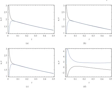
Figure 1:Solutions of linear stiffsystem fork 50, ε 0.01, α 1,aExact,bNumerical,c NHPM-Pade10/11,dNHPM-Pade10/11,k 50, ε 0.01, α 0.5color figure can be viewed in the online issue.

5. Concluding Remarks

The NHPM for solving system of fractional-order differential equations are based on two component procedure and polynomial initial condition. The NHPM applied on fractional-order Stiff equation, fractional Genesio equation, and the matrix Riccati-type differential equation. The Applications in problems 1–4 are plotted in Figures 1, 2, 3, and 4, which show the accuracy of NHPM. The computations associated with the applications discussed above, were performed by MATHEMATICA. The NHPM is very simple in application and is less computational more accurate in comparison with other mentioned methods. By using this method, the solution can be obtained in bigger interval. Unlike the ADM

0 0.5 1 1.5 2 2.5 3

−4

−6

−2 0 2 6 4

t

u,

v

a

0 0.5 1 1.5 2 2.5 3

−2

−4 0 2 4

t

u,

v

b

0 0.5 1 1.5 2 2.5 3

−5

−10 0 5 10

t

u,

v

c

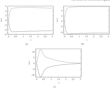
Figure 4:Solutions of matrix Riccati equationsu w,v zforα 1aNumerical,bNHPM-Pade

9/11,cNHPM-Pade9/11,α 0.5color figure can be viewed in the online issue.

Acknowledgment

M. Jamil is highly thankful and grateful to the Abdus Salam School of Mathematical Sciences, GC University, Lahore, Pakistan, the Department of Mathematics & Basic Sciences, NED University of Engineering & Technology, Karachi-75270, Pakistan, and also the Higher Education Commission of Pakistan for generously supporting and facilitating this research work.

References

1 H. M. Kilbas, H. M. Srivastava, and J. J. Trujillo, Theory and Applications of Fractional Differential Equations, Elsevier, Amsterdam, The Netherlands, 2007.

2 R. L. Bagley and R. A. Calico, “Fractional order state equations for the control of viscoelastically damped structures,”Journal of Guidance, Control, and Dynamics, vol. 14, no. 2, pp. 304–311, 1991.

3 A. Mahmood, S. Parveen, A. Ara, and N. A. Khan, “Exact analytic solutions for the unsteady flow of a non-Newtonian fluid between two cylinders with fractional derivative model,”Communications in Nonlinear Science and Numerical Simulation, vol. 14, no. 8, pp. 3309–3319, 2009.

4 A. Mahmood, C. Fetecau, N. A. Khan, and M. Jamil, “Some exact solutions of the oscillatory motion of a generalized second grade fluid in an annular region of two cylinders,”Acta Mechanica Sinica, vol. 26, no. 4, pp. 541–550, 2010.

6 N. A. Khan, N.-U. Khan, A. Ara, and M. Jamil, “Approximate analytical solutionsof fractional reaction-diffusion equations,”Journal of King Saud University—Science. In press.

7 J.-H. He, “Homotopy perturbation technique,”Computer Methods in Applied Mechanics and Engineering, vol. 178, no. 3-4, pp. 257–262, 1999.

8 J.-H. He, “A coupling method of a homotopy technique and a perturbation technique for non-linear problems,”International Journal of Non-Linear Mechanics, vol. 35, no. 1, pp. 37–43, 2000.

9 J.-H. He, “Homotopy perturbation method: a new nonlinear analytical technique,” Applied Mathematics and Computation, vol. 135, no. 1, pp. 73–79, 2003.

10 N. A. Khan, A. Ara, and A. Mahmood, “Approximate solution of time-fractional chemical engineering equations: a comparative study,”International Journal of Chemical Reactor Engineering, vol. 8, article A19, 2010.

11 N. A. Khan, N.-U. Khan, M. Ayaz, and A. Mahmood, “Analytical methods for solving the time-fractional Swift-HohenbergS-Hequation,”Computers and Mathematics with Applications. In press.

12 N. A. Khan, A. Ara, S. A. Ali, and M. Jamil, “Orthognal flow impinging on a wall with suction or blowing,”International Journal of Chemical Reactor Engineering. In press.

13 A. Yıldırım, “Solution of BVPs for fourth-order integro-differential equations by using homotopy perturbation method,”Computers & Mathematics with Applications, vol. 56, no. 12, pp. 3175–3180, 2008.

14 H. Koc¸ak, T. ¨Ozis¸, and A. Yıldırım, “Homotopy perturbation method for the nonlinear dispersive Km,n,1 equations with fractional time derivatives,”International Journal of Numerical Methods for Heat & Fluid Flow, vol. 20, no. 2, pp. 174–185, 2010.

15 Y. Khan, N. Faraz, A. Yildirim, and Q. Wu, “A series solution of the long porous slider,”Tribology Transactions, vol. 54, no. 2, pp. 187–191, 2011.

16 N. A. Khan, A. Ara, S. A. Ali, and A. Mahmood, “Analytical study of Navier-Stokes equation with fractional orders using He’s homotopy perturbation and variational iteration methods,”International Journal of Nonlinear Sciences and Numerical Simulation, vol. 10, no. 9, pp. 1127–1134, 2009.

17 H. Aminikhah and J. Biazar, “A new HPM for ordinary differential equations,”Numerical Methods for Partial Differential Equations, vol. 26, no. 2, pp. 480–489, 2010.

18 H. Aminikhah and M. Hemmatnezhad, “An efficient method for quadratic Riccati differential equation,”Communications in Nonlinear Science and Numerical Simulation, vol. 15, no. 4, pp. 835–839, 2010.

19 Y. Khan and N. Faraz, “Modified fractional decomposition method having integral w.r.t dξα,”

Journal of King Saud University—Science. In press.