On the difference equation \(x {n+1}=ax {n l}+bx {n k}+f ( x {n l},x {n k} )\)

R E S E A R C H

Open Access

On the difference equation

x

_n

₊₁

=

ax

_n

_–

_l

+

bx

_n

_–

_k

+

f

(

x

_n

_–

_l

,

x

_n

_–

_k

)

Mahmoud A.E. Abdelrahman

_{, George E. Chatzarakis}

_{, Tongxing Li}

_{and Osama Moaaz}

*_{Correspondence:}

4_{School of Information Science and}

Engineering, Linyi University, Linyi, P.R. China

Full list of author information is available at the end of the article

Abstract

In this paper, we study the asymptotic behavior of the solutions of a new class of difference equations

xn+1=axn–l+bxn–k+f(xn–l,xn–k),

wherelandkare nonnegative integers,aandbare nonnegative real numbers, the initial valuesx–s,x–s+1,. . .,x0are positive real numbers,s= max{l,k}, and

f(u,v) : (0,∞)2→(0,∞) is a continuous and homogeneous real function of degree zero. We consider the stability, boundedness, and periodicity of the solutions of this equation which is the most general form of linear difference equations. Thus, the results in this paper apply to several other equations that are special cases of the studied equation. Moreover, we present a new method to study periodic solutions of period two.

MSC: 39A10; 39A23; 39A30

Keywords: Difference equation; Equilibrium point; Local stability; Periodic solution

1 Introduction

Difference equations describe the observed evolution of a phenomenon at discrete time steps. Thus, difference equations are used as discrete models of the workings of physical or artificial systems. The asymptotic behavior of the solutions of linear difference equations is a qualitative property having important applications in many areas, including control theory, mathematical biology, neural networks, and so forth. We cannot use numerical methods to study the asymptotic behavior of all solutions of a given equation due to the global nature of that behavior. Therefore, the analytical study of those qualitative proper-ties has been attracting considerable interest from mathematicians and engineers, as the only method to gain insight into those properties.

This paper is concerned with the study of the asymptotic behavior of the solutions of a general class of difference equations

xn+1=axn–l+bxn–k+f(xn–l,xn–k), (1.1)

where l and k are nonnegative integers, a and b are nonnegative real numbers, and

f(u,v) : (0,∞)2_{→(0,∞) is a continuous and homogeneous real function of degree zero.}

The construction of this new class of difference equations is complex and involves several cases. For example, one can assumea= 0 orb= 0 or both. That makes our analysis better suited for studying those equations. For studies on equations of a similar form, the reader is referred to [1–25]. We begin our study with a review of the background on equations having a similar form to the one we consider in this paper.

Kalabušić and Kulenović [15] and Kulenović and Ladas [18] studied the difference equa-tion

xn+1=

a1xn–l+a2xn–k

b1xn–l+b2xn–k

.

Elsayed [12] investigated the asymptotic behavior of the difference equation

xn+1=A+

a1xn–l+a2xn–k

b1xn–l+b2xn–k

.

Zayed and El-Moneam [26,27,29] studied the asymptotic behavior of the difference equa-tion

xn+1=Axn+

a1xn+a2xn–k

b1xn+b2xn–k

,

whereas Zayed and El-Moneam [28] studied the global and asymptotic properties of the solutions of the difference equation

xn+1=Axn+Bxn–k+

a1xn+a2xn–k

b1xn+b2xn–k

.

Notice that these equations as well as several other equations not listed above are special cases of equation (1.1).

The results in this paper make three main contributions to the study of linear difference equations. First, we formulate a general class of difference equations as a means of estab-lishing general theorems for the asymptotic behavior of its solutions and the solutions of equations that are special cases of the studied equation. Second, we study the asymptotic behavior of the solutions of this more general class of difference equations using an effi-cient method introduced in [12] and modified in [19]. Theorem3.2establishes how this method can be applied to equation (1.1). In particular, this method is also valid and can be applied to several classes of difference equations for which the classical method fails to give results. Moreover, we consider difference equations with real coefficients and initial values which extend and slightly improve previous results. Third, we can use our analysis to check and verify the results obtained by other researchers.

For the basic definitions and auxiliary lemmas we use for establishing our results, namely equilibrium points, local stability, and periodicity of the solutions, we refer the reader to [1,9,17,18]. For the convenience of the reader, we present below some related results.

Lemma 1.1(see [17, Theorem 1.3.7]) Assume that p,q∈Rand k∈ {0, 1, 2, . . .}.Then|p|+

|q|< 1is a sufficient condition for the asymptotic stability of the difference equation

Lemma 1.2(see [9, Corollary 4]) Let f :Rn

+→Rbe continuous and differentiable onRn++.

If f is homogeneous of degree k,then Djf =∂f/∂xjis homogeneous of degree k– 1.

The rest of the paper is organized as follows. In Sect.2, we study the stability behav-ior and boundedness of the solutions of equation (1.1) and give an illustrative example in support of our analysis. In Sect.3, we present a technique to investigate the periodic behavior of the solutions of equation (1.1). A distinguishing feature of our criteria is that the coefficientslandkof equation (1.1) can be odd or even. Two examples are provided to illustrate the new method for studying periodic solutions. In Sect.4, the practicability, maneuverability, and efficiency of the results obtained are illustrated via two applications.

2 Dynamics of equation (1.1) 2.1 Local stability

Here, we investigate the local stability of the equilibrium point of equation (1.1), which is given by

x=ax+bx+f(x,x).

Hence, the positive equilibrium point is

x= 1

1 –a–bf(1, 1), a+b< 1.

Now, we define the functionφ(u,v) : (0,∞)2_{→(0,∞) by}

φ(u,v) =au+bv+f(u,v)

so that

∂φ

∂u(u,v) =a+fu(u,v),

∂φ

∂v(u,v) =b+fv(u,v).

Theorem 2.1 The equilibrium point of equation(1.1)x= (1 –a–b)–1_{f(1, 1)is locally}

asymptotically stable if

|ρ|–ρ< (1 –a–b)f(1, 1),

where

ρ=

⎧ ⎨ ⎩

bf(1, 1) – (1 –a–b)fu(1, 1) if fu> 0,

af(1, 1) – (1 –a–b)fv(1, 1) if fu< 0.

Proof The linearized equation of equation (1.1) aboutxis the linear difference equation

yn+1– ∂φ

∂u(x,x)yn–l–

∂φ

Hence, by Lemma1.1, equation (1.1) is locally stable if

∂φ_∂u(x,x)+∂φ ∂v(x,x)

< 1.

Therefore,

a+fu(x,x)+b+fv(x,x)< 1. (2.1)

From Euler’s homogeneous function theorem, we deduce thatufu= –vfvand thusfufv< 0.

Iffu> 0, then

b–fu(x,x)< 1 –a–fu(x,x).

Using Lemma1.2, we get

b–1

xfu(1, 1)

< 1 –a–1

xfu(1, 1),

which implies that inequality (2.1) is equivalent to

_{1 –}b_a–bf(1, 1) –fu(1, 1)

< 1 –a

1 –a–bf(1, 1) –fu(1, 1),

and so

bf(1, 1) – (1 –a–b)fu(1, 1)< (1 –a)f(1, 1) – (1 –a–b)fu(1, 1).

Next, iffu< 0, then

a–fv(x,x)< 1 –b–fv(x,x).

Similarly, we find

af(1, 1) – (1 –a–b)fv(1, 1)< (1 –b)f(1, 1) – (1 –a–b)fv(1, 1),

which completes the proof.

Example2.1 Consider the difference equation

xn+1=axn–l+bxn–k+c

xn–l

xn–k

, (2.2)

wherecis a positive real number. Note thatf(u,v) =cu/v. By Theorem2.1, the equilibrium point of equation (2.2)x=c/(1 –a–b) is locally asymptotically stable if

b– (1 –a–b)<b.

For example, forl= 0,k= 1,a= 0.2,b= 0.3,c= 1,x–1= 2.8, andx0= 1.5, the stable solution

Figure 1Stable solution corresponding to difference equation (2.2)

2.2 Boundedness

In this section, we study the boundedness of the solutions of equation (1.1).

Theorem 2.2 If a+b< 1and there exists a positive constant L such that f(u,v) <L for all u,v∈(0,∞),then every solution of equation(1.1)is bounded.

Proof From equation (1.1), we obtain

xn+1=axn–l+bxn–k+f(xn–l,xn–k)

<axn–l+bxn–k+L.

Using a comparison, we can write the right-hand side as follows:

yn+1=ayn–l+byn–k+L,

and this equation is locally stable ifa+b< 1 and converges to the equilibrium pointy=

L/(1 –a–b). Then we havexn<ynand

lim sup

n→∞ xn≤

L

1 –a–b.

Thus, every solution of (1.1) is bounded.

Remark2.3 As fairly noticed by the referees, the global asymptotic stability of equation (1.1) remains an open problem for further research.

3 Periodic solutions

Theorem 3.1 If l and k are either odd or even,then equation(1.1)has no solutions of prime period two.

Proof Suppose thatlandkare even and equation (1.1) has a prime period two solution

Thenxn–l=xn–k=q. From equation (1.1), we have

p= (a+b)q+f(q,q),

q= (a+b)p+f(p,p).

Thus, we get

p=q= 1 +a+b 1 – (a+b)2f(1, 1),

which is a contradiction. Another case can be shown similarly. This completes the proof.

Theorem 3.2 Assume that l is odd and k is even.Then equation(1.1)has a prime period two solution

. . . ,p,q,p,q, . . .

if and only if

(1 –a) –bτf(τ, 1) =(1 –a)τ–bf(1,τ), (3.1)

whereτ =p/q.

Proof Without loss of generality, we can assume thatl>k. Now, let equation (1.1) have a prime period two solution

. . . ,p,q,p,q, . . . .

Sincelis odd andkis even, we arrive atxn–l=pandxn–k=q. From equation (1.1), we get

p=ap+bq+f(p,q),

q=aq+bp+f(q,p).

This yields

(1 –a)p=bq+f(τ, 1),

(1 –a)q=bp+f(1,τ),

whereτ=p/q. Then we obtain

(1 –a)2–b2 p=bf(1,τ) + (1 –a)f(τ, 1),

(1 –a)2–b2 q=bf(τ, 1) + (1 –a)f(1,τ).

Sincep=τq, we find

On the other hand, suppose that (3.1) is satisfied. Now, we choose

x–l+2r=λf(1,τ) +μf(τ, 1) and

x–l+2r+1=λf(τ, 1) +μf(1,τ), r= 0, 1, 2, . . . , (l– 1)/2,

where

λ= b

(1 –a)2_–b2, μ=

1 –a

(1 –a)2_–b2,

andτ∈R+. Hence, we see that

x1=ax–l+bx–k+f(x–l,x–k)

=aλf(1,τ) +μf(τ, 1)+bλf(τ, 1) +μf(1,τ)

+fλf(1,τ) +μf(τ, 1),λf(τ, 1) +μf(1,τ) . (3.2)

From (3.1), we have

[μ–λτ]f(τ, 1) = [μτ–λ]f(1,τ),

and so

μf(τ, 1) +λf(1,τ) =τλf(τ, 1) +μf(1,τ),

which together with (3.2) implies that

x1=aλf(1,τ) +aμf(τ, 1) +bλf(τ, 1) +bμf(1,τ) +f(τ, 1)

= (aμ+bλ+ 1)f(τ, 1) + (aλ+bμ)f(1,τ)

=μf(τ, 1) +λf(1,τ).

Similarly, we can show thatx2=λf(τ, 1) +μf(1,τ). Then, by induction, we conclude that

x2n–1=μf(τ, 1) +λf(1,τ) and x2n=λf(τ, 1) +μf(1,τ) for alln> 0.

This completes the proof.

Theorem 3.3 Assume that l is even and k is odd.Then equation(1.1)has a prime period two solution

. . . ,p,q,p,q, . . .

if and only if

a– (1 –b)τf(τ, 1) =aτ– (1 –b)f(1,τ), (3.3)

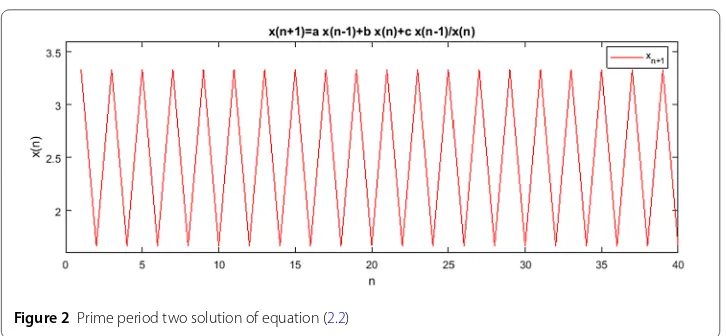
Figure 2Prime period two solution of equation (2.2)

Proof The proof is similar to that of Theorem3.2and thus is omitted.

Example3.1 Consider equation (2.2) and assume thatlis odd andkis even. By virtue of Theorem3.2, equation (2.2) has a prime period two solution

. . . ,p,q,p,q, . . .

if and only if

(τ– 1)b–τ+aτ+bτ+bτ2 = 0.

Sinceτ= 1, we obtain

1 +τ2

τ =

1 –a–b b .

Letting

H(τ) =1 +τ

2

τ >τmin∈R+H(τ) = 2 forτ∈R

+_\{1},

we geta+ 3b< 1. For a numerical example, we takel= 1,k= 0, a= 0.3,b= 0.2,c= 1,

x–1= 3.3333, andx0= 1.6667; see Fig.2.

Remark3.4 Consider the equation

xn+1=axn+bxn–k+

pxn+xn–k

qxn+xn–k

, (3.4)

which was studied by Zayed and El-Moneam [28]. Define the function

f(u,v) =pu+v

qu+v.

Thenf is homogeneous with degree zero and

fu(u,v) =

(p–q)v

(qu+v)2 and fv(u,v) =

(q–p)u

From Theorem2.1, the positive equilibrium point of equation (3.4) is

x= 1 1 –a–b

p+ 1

q+ 1.

This point is asymptotically stable ifp>qand

prime period two solutions. Furthermore, using Theorem3.3, ifkis odd, then equation (3.4) has a prime period two solution if and only if

Remark3.5 Several equations that have been studied in [26,27,29] can be treated as spe-cial cases of (1.1).

4 Applications

4.1 Application 1

wheref is homogeneous with degree zero and

fu(u,v) =

Note thatfu> 0. Then, by Theorem2.1, the positive equilibrium point

x= 1

of equation (4.1) is locally asymptotically stable if

β

Figure 3Stable solution of difference equation (4.1)

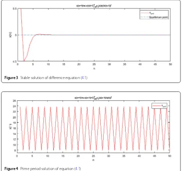
Figure 4Prime period solution of equation (4.1)

Then, we get β_i=1(2i– 1)ci<c0. For a numerical example, we takel= 1,k= 0,β= 2,

a= 0.1,c0= 19/3,c1= 2,c2= 1,x–1= 23.704, andx0= 7.9012; see Fig.4.

Conjecture 1 Note that, ifβ_i=1(2i– 1)ci<c0, then every solution of equation (4.1)

con-verges either to the equilibrium point or to a periodic solution having period two.

4.2 Application 2

Consider the difference equation

xn+1=axn–l+bxn–k+e–cxn–l/xn–k, (4.2)

wherecis a real number. Forc> 0, define the function

f(u,v) =e–cu/v,

which is homogeneous with degree zero and

fu(u,v) = –

c ve

–cu/v_{< 0,}

fv(u,v) =

cu v2e

Figure 5Stable solution of difference equation (4.2)

Figure 6Prime period solution of equation (4.2)

By Theorem2.1, the positive equilibrium point of equation (4.2)

x= e

–c

1 –a–b

is locally asymptotically stable if

a– (1 –a–b)c–a– (1 –a–b)c < 1 –a–b.

Then

a> (1 –a–b)c

or

(1 –a–b)(2c– 1) < 2a.

For a numerical example, we takel= 0,k= 1,a= 0.8,b= 0.1,c= 1,x–1= 5, andx0= 5.9;

Letl be odd andk be even. By Theorem3.2, equation (4.2) has a prime period two

The authors express their sincere gratitude to the editors and two anonymous referees for the careful reading of the original manuscript and useful comments that helped to improve the presentation of the results and accentuate important details.

Funding

This research is supported by NNSF of P.R. China (Grant No. 61503171), CPSF (Grant No. 2015M582091), NSF of Shandong Province (Grant No. ZR2016JL021), KRDP of Shandong Province (Grant No. 2017CXGC0701), DSRF of Linyi University (Grant No. LYDX2015BS001), and the AMEP of Linyi University, P.R. China.

Availability of data and materials

Data sharing not applicable to this article as no datasets were generated or analysed during the current study.

Competing interests

The authors declare that they have no competing interests.

Authors’ contributions

All four authors contributed equally to this work. They all read and approved the final version of the manuscript.

Author details

1_{Department of Mathematics, Faculty of Science, Mansoura University, Mansoura, Egypt.}2_{Department of Electrical and}

Electronic Engineering Educators, School of Pedagogical and Technological Education (ASPETE), Athens, Greece.3_LinDa

Institute of Shandong Provincial Key Laboratory of Network Based Intelligent Computing, Linyi University, Linyi, P.R. China.

4_{School of Information Science and Engineering, Linyi University, Linyi, P.R. China.}

Publisher’s Note

Springer Nature remains neutral with regard to jurisdictional claims in published maps and institutional affiliations.

Received: 17 February 2018 Accepted: 8 November 2018

References

1. Abdelrahman, M.A.E., Moaaz, O.: Investigation of the new class of the nonlinear rational difference equations. Fundam. Res. Dev. Int.7(1), 59–72 (2017)

2. Abo-Zeid, R.: Attractivity of two nonlinear third order difference equations. J. Egypt. Math. Soc.21(3), 241–247 (2013) 3. Abo-Zeid, R.: On the oscillation of a third order rational difference equation. J. Egypt. Math. Soc.23(1), 62–66 (2015) 4. Abu-Saris, R.M., DeVault, R.: Global stability ofyn+1=A+_yn–kyn . Appl. Math. Lett.16(2), 173–178 (2003)

5. Amleh, A.M., Grove, E.A., Ladas, G., Georgiou, D.A.: On the recursive sequencexn+1=α+xn–1/xn. J. Math. Anal. Appl.

233(2), 790–798 (1999)

6. Berenhaut, K.S., Foley, J.D., Stevi´c, S.: The global attractivity of the rational difference equationyn= 1 +_yn–myn–k. Proc. Am.

Math. Soc.135(4), 1133–1140 (2007)

7. Berenhaut, K.S., Stevi´c, S.: A note on positive non-oscillatory solutions of the difference equationxn+1=α+ xp_n–k

xp_n .

J. Differ. Equ. Appl.12(5), 495–499 (2006)

8. Berenhaut, K.S., Stevi´c, S.: The behaviour of the positive solutions of the difference equationxn=A+ (xn–2_xn–1)p. J. Differ.

Equ. Appl.12(9), 909–918 (2006)

9. Border, K.C.: Euler’s theorem for homogeneous functions (2000)

http://www.its.caltech.edu/~kcborder/Notes/EulerHomogeneity.pdf

10. DeVault, R., Kent, C., Kosmala, W.: On the recursive sequencexn+1=p+xn–k_xn . J. Differ. Equ. Appl.9(8), 721–730 (2003)

11. DeVault, R., Ladas, G., Schultz, S.W.: On the recursive sequencexn+1=_xnA +_xn–21 . Proc. Am. Math. Soc.126(11),

12. Elsayed, E.M.: New method to obtain periodic solutions of period two and three of a rational difference equation. Nonlinear Dyn.79(1), 241–250 (2015)

13. Grove, E.A., Ladas, G.: Periodicities in Nonlinear Difference Equations, vol. 4. Chapman & Hall/CRC, Boca Raton (2005) 14. Hamza, A.E.: On the recursive sequencexn+1=α+xn–1/xn. J. Math. Anal. Appl.322(2), 668–674 (2006)

15. Kalabuši´c, S., Kulenovi´c, M.R.S.: On the recursive sequencexn+1=γ_{Cxn–1 +Dxn–2}xn–1 +δxn–2. J. Differ. Equ. Appl.9(8), 701–720 (2003)

16. Khuong, V.V.: On the positive nonoscillatory solution of the difference equationsxn+1=α+ (xn–k/xn–m)p. Appl. Math. J.

Chin. Univ. Ser. B24, 45–48 (2009)

17. Kocic, V.L., Ladas, G.: Global Behavior of Nonlinear Difference Equations of Higher Order with Applications. Kluwer Academic Publishers, Dordrecht (1993)

18. Kulenovi´c, M.R.S., Ladas, G.: Dynamics of Second Order Rational Difference Equations with Open Problems and Conjectures. Chapman & Hall/CRC, Boca Raton (2002)

19. Moaaz, O.: Comment on “New method to obtain periodic solutions of period two and three of a rational difference equation” [Nonlinear Dyn. 79: 241–250]. Nonlinear Dyn.88(2), 1043–1049 (2017)

20. Moaaz, O., Abdelrahman, M.A.E.: Behaviour of the new class of the rational difference equations. Electron. J. Math. Anal. Appl.4(2), 129–138 (2016)

21. Öcalan, Ö.: Dynamics of the difference equationxn+1=pn+xn–k_xn with a period-two coefficient. Appl. Math. Comput.

228, 31–37 (2014)

22. Saleh, M., Aloqeili, M.: On the rational difference equationyn+1=A+yn–k_yn . Appl. Math. Comput.171(2), 862–869

(2005)

23. Stevi´c, S.: On the recursive sequencexn+1=α+ xp_n–1

xpn

. J. Appl. Math. Comput.18(1–2), 229–234 (2005)

24. Sun, T., Xi, H.: On convergence of the solutions of the difference equationxn+1= 1 +xn–1_xn . J. Math. Anal. Appl.325(2),

1491–1494 (2007)

25. Yan, X.-X., Li, W.-T., Zhao, Z.: On the recursive sequencexn+1=α– (xn/xn–1). J. Appl. Math. Comput.17(1–2), 269–282

(2005)

26. Zayed, E.M.E., El-Moneam, M.A.: On the rational recursive sequencexn+1=Axn+ (βxn+γxn–k)/(Cxn+Dxn–k). Commun.

Appl. Nonlinear Anal.16(3), 91–106 (2009)

27. Zayed, E.M.E., El-Moneam, M.A.: On the rational recursive sequencexn+1=γxn–k+ (axn+bxn–k)/(cxn–dxn–k). Bull. Iran.

Math. Soc.36(1), 103–115 (2010)

28. Zayed, E.M.E., El-Moneam, M.A.: On the rational recursive sequencexn+1=Axn+Bxn–k+β_Cxn+xn+γ_Dxn–kxn–k. Acta Appl. Math.

111(3), 287–301 (2010)

29. Zayed, E.M.E., El-Moneam, M.A.: On the rational recursive two sequencesxn+1=axn–k+bxn–k/(cxn+δdxn–k). Acta Math.