R E S E A R C H
Open Access
New upper and lower bounds, the
iteration algorithm for the solution of the
discrete algebraic Riccati equation
Juan Zhang and Jianzhou Liu
**Correspondence: [email protected]
Department of Mathematics and Computational Science, Xiangtan University, Xiangtan, Hunan 411105, P.R. China
Abstract
In this paper, applying the properties of matrix Schur complement and matrix inverse, via some matrix equalities and inequalities, we present new lower and upper solution bounds of the discrete algebraic Riccati equation. Then, by the compressed image principle and a matrix norm inequality, we offer an existence uniqueness condition and a fixed point iteration algorithm for the solution of the discrete algebraic Riccati equation. Finally, a corresponding numerical example demonstrates the effectiveness of the developed results.
Keywords: matrix bound; discrete algebraic Riccati equation; Schur complement; eigenvalue
1 Introduction and preliminaries
The discrete algebraic Riccati equation has many applications in the process of obtaining optimal control and determining system stability [, ]. For example, consider the follow-ing linear discrete system (see []):
x(t+ ) =Ax(t) +Bu(t), (.)
wherex(t)∈Rnis the state variable,u(t)∈Rmis the input variable,A∈Rn×nis the system
matrix,B∈Rn×mis the input matrix.
The system (.) is associated with the linear quadratic optimal control problem of min-imizing the quadratic performance index
J=
∞
t=
x(t)
u(t)
T
Q ST
S G x(t)
u(t)
,
whereS∈Rm×n,G∈Rm×m,Q∈Rn×nare symmetric positive definite matrices, then the
problem switches to how to solve the symmetric positive definite solutionP∈Rn×nof the
following equation:
P=ATPA+Q–ATPB+STG+BTPB–BTPA+S. (.)
IfS= ,G=Im, (.) becomes the discrete algebraic Riccati matrix equation
P=ATPA–ATPBI+BTPB–BTPA+Q. (.)
In many practical control problems, to study the discrete algebraic Riccati equation (.),
we usually assume thatQis positive semi-definite. When considering certainH-infinity
problems and LQG problems and so on in some discrete control linear systems, the as-sumption thatQis positive definite is only required. Certainly, it is difficult to discuss this equation on the assumption thatQis positive semi-definite. Thus, there are many scholars to research this equation on the assumption thatQis positive definite [–].
As the discrete algebraic Riccati equations (.) and (.) play an important role in many control analysis and design problems (Bernstein, []; Kojimaet al., []), dis-cussing these equations becomes a heated topic. For one thing, it is important to solve these equations (Kojimaet al., []). It is difficult to obtain their solutions, and there are few iterative algorithms for getting the solutions of these equations (Komaroff, []). Reference [] derives the iterative solution algorithm on the assumption that for the discrete algebraic Riccati equations (.) there exists a positive definite solution. In certain control problems, if the original system is assumed to be stabilizable, the exact solutions of the discrete algebraic Riccati equations (.) and (.) are not often required, while a reasonably tight solution bound will only be required such as the stabilization of jump linear systems (Fang and Loparo, []) and the quadratic optimization problem for a class of singularly perturbed stochastic systems (Dragan, []). Hence, in recent years, many researchers paid much attention to studying the discrete algebraic Riccati equations (.) and (.). Those include a recursive solution (Assimakiset al., []), a matrix inequality (Saberi, []), prediction, estimation, and smoothing error covariance ma-trices (Assimakis and Adam, []), iterative and algebraic algorithms (Assimakis and Adam, []; Chianget al., []), matrix bounds (Choi, []; Kim and Park, []; Gaoet al., []; Komaroff, , [, ]; Lee and Chang, []; Lee, , , [–], Liu and Zhang, , [–], Zhang and Liu, [, ]), eigenvalue bounds (Garloff, []; Lee, []), trace bounds (Kimet al., []), summation bounds (Komaroff and Shahian, []), norm bounds (Patel and Toda, []), and perturbation bounds (Hasanovet al., []; Hasanov, []). The most general bounds are the solution bounds, as they can directly offer the other types of bounds mentioned. Thus, based on the above, there are three problems to be considered as follows:
() When does there exist a positive definite solution of the discrete algebraic Riccati equation (.)?
() If the discrete algebraic Riccati equation (.) possesses a positive definite solution under certain conditions, in what range is the solution unique? In addition, how do we estimate the upper and lower solution bounds of this equation?
() If the discrete algebraic Riccati equation (.) possesses a unique positive definite solution in a certain range, how do we design the iterative solution algorithms? Further, we need to discuss the solution bounds affecting the iterative algorithms.
(.). Finally, a corresponding numerical example demonstrates the effectiveness of the developed results.
Throughout this paper, we use the following symbol conventions. LetRn×mandN+ de-note the set ofn×mreal matrices and positive integers. ForX= (xij)∈Rm×n, letXT,X
denote the transpose and the spectral norm ofX, respectively. IfX∈Rn×n,X–denotes the
inverse ofX. IfX,Y∈Rn×n, the inequalityX> (≥) means thatXis a symmetric positive
(semi-) definite matrix and the inequalityX> (≥)YmeansX–Yis a symmetric positive
(semi-) definite matrix. SupposeX∈Rn×nis an arbitrary symmetric matrix, we assume
that the eigenvalues ofXare arranged so thatλ(X)≥λ(X)≥ · · · ≥λn(X). ForX∈Rn×n,
suppose the singular values ofXare arranged so thatσ(X)≥σ(X)≥ · · · ≥σn(X). The
identity matrix with appropriate dimensions is represented byI.
LetN={, , . . . ,n}. For nonempty index setsα,β⊆N whose elements are both con-ventionally arranged in increasing order, we denote by |α| the cardinality ofα and by
αc=N–αthe complement ofαinN. We writeX(α,β) to mean the submatrix ofX∈Rn×n
lying in the rows indexed byα and the columns indexed byβ.X(α,α) is abbreviated to
X(α). Assuming thatX(α) is nonsingular, denote the Schur complement with respect to
X(α) by
X/α=X/X(α) =Xαc–Xαc,αX(α) –Xα,αc.
The following lemmas are used to prove the main results.
Lemma .(Zhang [], p., Theorem .) Let X∈Rn×nbe partitioned as
X=
E F G H
,
and suppose both X and E∈Rm×mare nonsingular matrices.Then X/E is nonsingular and
X–=
E–+E–FS–GE– –E–FS–
–S–GE– S–
,
where S=H–GE–F=X/E.
Lemma .(Zhang [], p., Case ) If the matrix X is defined as Lemma.,choosing
α={, , . . . ,m},then
(X/α)–=X–αc.
Lemma .(Lee []) Let P be the positive semi-definite solution of the discrete algebraic Riccati equation(.),andσ
(A) < +σn(B)δ,then P has the upper matrix bound P≤ λ(Q)
+δσn(B) –σ(A)
ATA+Q≡η, (.)
Definition . (Rudin []) The pair (X,d) is called a complete metric space ifXis a nonempty set whose elements are denoted byx,y, . . . and assume that on the Cartesian productX×Xa distance functiondis defined satisfying the following conditions:
(D) d(x,y)≥,
(Dl) d(x,y) = if and only ifx=y, (D) d(x,y) =d(y,x),
(D) d(x,y)≤d(x,z) +d(z,y),
(D) everyd-Cauchy sequence inXisd-convergent,i.e., ifxnis a sequence inXsuch
thatlimn,m→∞d(xn,xm) = , then there is anx∈Xwithlimn→∞d(xn,x) = .
Definition .(Rudin []) The pair (X, · ) is called a normed space ifXis a real vector space whose elements are denoted byx,y,z, . . . and assume that for everyx∈Xthere is associated a nonnegative real numberx, called the norm ofx, in such a way that:
(D) x+y ≤ x+y,
(Dl) αx=|α| · xwhereαis a scalar, (D) x> ifx= .
Lemma .(Berinde [], Theorem B) Let(X,d)be a complete metric space and F:X−→ X be a strict contraction,i.e.,a map satisfying
d(Fx,Fy)≤ad(x,y), for all x,y∈X,
where≤a< is constant.Then F has a unique fixed point in X.
Every normed space may be regarded as a metric space, in which the distanced(x,y)
betweenxandyisx–y. Hence, we get the following conclusion from Definitions .,
. and Lemma ..
Lemma . Let(X, · ) be a real Banach space, and⊂X be a convex,closed and
bounded subset and F:−→be a contraction map,i.e.,a map satisfying F(P) –F(P)≤pP–P, for all P,P∈,
where≤p< is constant.Then F has a unique fixed point in.
Lemma .(Zhaoet al.[], Lemma .) If X,Y∈Rn×n,and <X≤Y,then X ≤ Y.
2 New solution bounds for the discrete algebraic Riccati equation (1.3)
In this section, we first present a lemma (Lemma .). Then new lower and upper solution bounds are deduced from Lemma ..
Lemma . Define the map
then
Applying Lemma . to (.) yields
Q=
Introducing Lemma . to (.) gives
Q–=F(P)–+F(P)–ATP–+BBT–AF(P)–AT –AF(P)–. (.)
from which one infers that
In terms of (.), it is evident that
Combining (.) with (.) shows that
F(P) –
Substituting (.) into (.) gives
F(P) =Q
which completes the proof.
Theorem . Let P be the positive definite solution of the discrete algebraic Riccati equa-tion(.),then P has the lower matrix bound
P≥Q
Proof From (.), we have
P=ATPP––BI+BTPB–BT PA+Q. (.)
according to Lemmas . and ., (.) changes to
Since
This completes the proof.
Furthermore, we propose new lower and upper solution bounds on the basis of Lem-ma ..
Proof Applying Lemma . and (.) to (.), it is simple to see that
This completes the proof.
Remark . For one thing, we point out thatP≥P≥Q. Indeed,
Remark . Pandηare two different upper bounds. It is difficult to compare them for
the same measure. Further, in Section , we offer a numerical example which shows that
Pis better thanη(i.e.,P≤η) in a certain case. It is hard to prove that this result holds
for the general case in the theory.
3 On the solution existence uniqueness of the discrete algebraic Riccati equation (1.3)
Theorem . Letσ
we getP≤P. Suppose the discrete algebraic Riccati equation (.) possesses a positive
definite solution, from Theorem ., then the positive definite solution is in [P,P],i.e.,
Thus, by Lemma ., we obtain
Consequently, forP∈, we getP≤F(P)≤P.
ThusF()⊆. For arbitraryP,P∈,
F(P) =AT
P– +BBT–A+Q,
F(P) =AT
P– +BBT–A+Q. Consequently,
F(P) –F(P) =AT
P–+BBT––P– +BBT– A
=ATP–+BBT–P– +BBT–P– +BBT P– +BBT–A
=ATP–+BBT–P––P–P– +BBT–A
=ATP–+BBT–P– (P–P)P–
P–+BBT–A. SinceP≤P≤P, according to Lemma ., we have
F(P) –F(P)=AT
P–+BBT–P–(P–P)P–
P– +BBT–A ≤AT· A ·P– ·P–·P– +BBT–
·P– +BBT–· P–P
≤AT· A ·P– ·P–·P– +BBT– ·P– +BBT–· P–P
=A·P– ·P– +BBT–· P–P
=pP–P. (.)
Asp< , thus the mapF(P) is a contraction map in. In the light of Lemma ., the map
F(P) has a unique fixed point in.
Combing () and () shows that (.) has a unique positive definite solutionP, andP≤
P≤P.
4 A fixed point iteration algorithm for the solution of the discrete algebraic Riccati equation (1.3)
In this section, based on Theorem ., we present a fixed point iteration algorithm for the solution of the discrete algebraic Riccati equation (.).
For arbitrary givenP()∈={P|P
≤P≤P}, we construct the matrix sequence
P(k+)=ATP(k)–+BBT –A+Q, k= , , . . . . (.)
Next, we prove P(k) is convergent and converges to the exact solution of the discrete
algebraic Riccati equation (.).
Theorem . If the conditions of Theorem.are satisfied,then the sequence P(k)given by
Proof ForP()∈, in terms of (.), fork∈N+, we obtain a sequence{P(k)}, then
P(k)–P(k–)=ATP(k–)–+BBT ––P(k–)–+BBT –A
=ATP(k–)–+BBT –P(k–)–+BBT –P(k–)–+BBT ×P(k–)–+BBT –A
=ATP(k–)–+BBT –P(k–)––P(k–)– P(k–)–+BBT –A
=ATP(k–)–+BBT –P(k–)–P(k–)–P(k–)P(k–)– ×P(k–)–+BBT –A.
In a similar way to the proof of (.), we obtain
P(k)–P(k–)≤pP(k–)–P(k–).
Applying mathematical induction, it is easy to get
P(k)–P(k–)≤pk–P()–P(). (.)
Because <p< , thuslimk→∞pk= . Then,∀ε> ,∃N
∈N+,∀k>N, we get
pk< ε( –p)
P()–P(). (.)
Consequently,∀k>N,∀v∈N+, using the triangular inequality, (.), and (.), we obtain P(k+v)–P(k)≤P(k+v)–P(k+v–)+P(k+v–)–P(k+v–)+· · ·+P(k+)–P(k)
≤pk+v–+pk+v–+· · ·+pkP()–P()
= p
k–pk+v
–p P
()–P()
< p
k
–pP
()–P()
<ε.
HenceP(k)is a Cauchy sequence in, thenP(k)is convergent. Denotelimk→∞P(k)=P.
Letk→ ∞in (.), then
P=AT
P– +BBT–A+Q.
This shows thatPis a solution of (.). According to Theorem .,Pis the unique
pos-itive definite solution of the discrete algebraic Riccati equation (.). This completes the
proof.
By Theorem ., defineP(k)as thekth iterative solution of the discrete algebraic Riccati
have the error estimation
P(k+)–P(k)≤pkP()–P()≤pkP–P<ε.
In the case of the precisionεis permitted, we have the following algorithm.
Algorithm .
Input: For the discrete algebraic Riccati equation (.), givenA,B,Q. Output: P(k).
Step : ComputePandP.
Step : Computep, if <p< , go to Step ; otherwise, stop. Step : SetP()∈={P|P
≤P≤P}.
Step : Compute
P(k+)=ATP(k)–+BBT –A+Q, k= , , . . . .
Step : For any smallε> andk∈N+, ifP(k+)–P(k)<ε, stop; otherwise, letk=k+ ,
go to Step .
5 A numerical example
In this section, we demonstrate the effectiveness of our results by the following real appli-cation example. In many engineering fields such as solid mechanics, quantum mechanics, parameter identification and automatic control, we often need to study the system stabil-ity and optimal control of linear discrete systems. Sometimes, these problems reduce to discussing the symmetric positive definite solution of the corresponding discrete algebraic Riccati matrix equations (.) and (.). The whole process of the example is carried out on Matlab . and the precision is –.
Example . Consider the following linear discrete system (see []):
x(t+ ) =Ax(t) +Bu(t), (.)
wherex(t)∈Rnis the state variable,u(t)∈Rmis the input variable,A∈Rn×nis the system
matrix,B∈Rn×mis the input matrix. Here, we choose
A=
⎛ ⎜ ⎝
. . .
. .
. –. .
⎞ ⎟ ⎠,
B=
⎛ ⎜ ⎝
. .
. .
. .
⎞ ⎟ ⎠.
The quadratic performance index of (.) is
J=
∞
t=
where
Q=
⎛ ⎜ ⎝
. . .
. . .
. . .
⎞ ⎟ ⎠
is symmetric positive definite.
In order to seek the optimal control such that the quadratic performance index (.) attains the minimum, we use the minimum principle. Choose the Hamiltonian function as
H(t) = x
T(t)Qx(t) +
u
T(t)u(t) +χT(t+ )Ax(t) +Bu(t) .
Then we can obtain the canonical equation
χ(t) = ∂H(t)
∂x(t) =Qx(t) +A
Tχ(t+ ), (.)
and the control equation
∂H(t)
∂u(t) =u(t) +B
Tχ(t+ ) = ,
i.e.,
u(t) = –BTχ(t+ ). (.)
Suppose
χ(t) =Px(t). (.)
Substituting (.) into the canonical equation (.) yields
Px(t) =Qx(t) +ATPx(t+ ). (.)
Using the state equation (.) and the control equation (.), we have
x(t+ ) =Ax(t) +Bu(t) =Ax(t) –BBTPx(t+ ),
then
x(t+ ) =I+BBTP–Ax(t). (.)
Substituting (.) into (.), eliminatingx(t) on both sides of the equality, applying the Sherman-Morrison-Woodbury equality
we get the discrete algebraic Riccati equation (.),
P=ATPA–ATPBI+BTPB–BTPA+Q.
In terms of (.) and (.), by (.), we obtain the optimal control
u(t) = –I+BTPB–BTPAx(t) (.)
such that the quadratic performance index (.) attains a minimum, wherePis the
sym-metric positive definite solution of the discrete algebraic Riccati equation (.). Obviously,σ
(A) < +σn(B)δ, then the upper matrix bound for the solutionPof the
discrete algebraic Riccati equation (.) by (.) is
η=
The lower matrix bound for the solutionPof the discrete algebraic Riccati equation (.) found by (.) is
The lower and upper matrix bounds for the solutionPof the discrete algebraic Riccati equation (.) found by (.) are
leading to
λ(P) = ., λ(P) = .,
λ(P) = ..
Obviously,
P≥P, η≥P.
This shows that the lower boundPis better thanP, and the upper boundPis better
thanη.
By computation, obviously,P≤P,AT(P– +BBT)–A+Q≤η, and
<p= . < .
According to Theorem ., the discrete algebraic Riccati equation (.) has a unique pos-itive definite solutionP, andP≤P≤P.
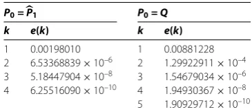
Lete(k) =P(k+)–P(k)be the iteration error at thekth iteration,kdenote the iteration
number, where we chooseε= – andP()=P
andP()=Q, respectively. Then
Algo-rithm . and Theorem . of [] need and iteration steps, respectively, to converge to the iteration solution of the discrete algebraic Riccati equation (.) as follows:
P=
⎛ ⎜ ⎝
. . .
. . .
. . .
⎞ ⎟ ⎠.
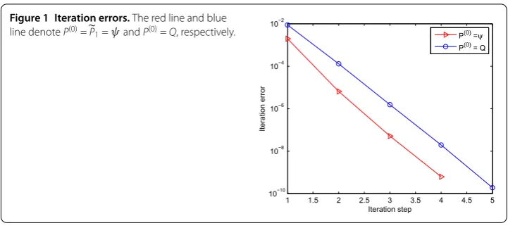
The relation between iteration step and iteration error is shown in Table and Figure . Obviously, Table and Figure show that compared to Theorem . of [], Algorithm . has less errors and less iteration steps.
Thus, by (.), we can have the optimal control
u(t) = –I+BTPB–BTPAx(t)
=
⎛ ⎜ ⎝
. . .
. . .
. . .
⎞ ⎟ ⎠x(t)
such that the quadratic performance index (.) attains a minimum.
Table 1 Iteration errors (ε= 10–8)
P0=P1 P0= Q
k e(k) k e(k)
1 0.00198010 1 0.00881228
2 6.53368839×10⁻⁶ 2 1.29922911×10⁻⁴
3 5.18447904×10⁻⁸ 3 1.54679034×10⁻⁶
4 6.25516090×10⁻¹⁰ 4 1.94930367×10⁻⁸
Figure 1 Iteration errors.The red line and blue line denoteP(0)=P
1=ψandP(0)=Q, respectively.
Competing interests
The authors declare that they have no competing interests.
Authors’ contributions
All authors contributed equally to the writing of this paper. All authors read and approved the final manuscript.
Acknowledgements
The work was supported in part by National Natural Science Foundation of China (11571292, 11471279), National Natural Science Foundation for Youths of China (11401505), the Key Project of National Natural Science Foundation of China (91430213), the General Project of Hunan Provincial Natural Science Foundation of China (2015JJ2134), and the General Project of Hunan Provincial Education Department of China (15C1320).
Received: 14 May 2015 Accepted: 28 September 2015
References
1. Bernstein, DS: Matrix Mathematics: Theory, Facts and Formulas with Application to Linear Systems Theory. Princeton University Press, Princeton (2005)
2. Kojima, C, Takaba, K, Kaneko, O, Rapisarda, P: A characterization of solutions of the discrete-time algebraic Riccati equation based on quadratic difference forms. Linear Algebra Appl.416, 1060-1082 (2006)
3. Komaroff, N: Iterative matrix bounds and computational solutions to the discrete algebraic Riccati equation. IEEE Trans. Autom. Control39, 1676-1678 (1994)
4. Lee, CH, Hsien, TL: New solution bounds for the discrete algebraic matrix Riccati equation. Optim. Control Appl. Methods20, 113-125 (1999)
5. Garloff, J: Bounds for the eigenvalues of the solution of the discrete Riccati and Lyapunov equations and the continuous Lyapunov equation. Int. J. Control43, 423-431 (1986)
6. Lee, CH: A unified approach to eigenvalue bounds of the solution of the Riccati equation. J. Chin. Inst. Eng.27, 431-437 (2004)
7. Fang, Y, Loparo, KA: Stabilization of continuous-time jump linear systems. IEEE Trans. Autom. Control47, 1590-1603 (2002)
8. Dragan, V: The linear quadratic optimization problem for a class of singularly stochastic systems. Int. J. Innov. Comput. Inf. Control1, 53-63 (2005)
9. Assimakis, N, Roulis, S, Lainiotis, D: Recursive solutions of the discrete time Riccati equation. Neural Parallel Sci. Comput.11, 343-350 (2003)
10. Saberi, SA: The discrete algebraic Riccati equation and linear matrix inequality. Linear Algebra Appl.274, 317-365 (1998)
11. Assimakis, N, Adam, M: Kalman filter Riccati equation for the prediction, estimation and smoothing error covariance matrices. ISRN Comput. Math.13, Article ID 249594 (2013). doi:10.1155/2013/249594
12. Assimakis, N, Adam, M: Iterative and algebraic algorithms for the computation of the steady state Kalman filter gain. ISRN Appl. Math.2014, Article ID 417623 (2014). doi:10.1155/2014/417623
13. Chiang, C-Y, Fan, H-Y, Lin, W-W: A structured doubling algorithm for discrete-time algebraic Riccati equations with singular control weighting matrices. Taiwan. J. Math.14(3A), 933-954 (2010)
14. Choi, HH: Upper matrix bounds for the discrete algebraic Riccati matrix equation. IEEE Trans. Autom. Control46, 504-508 (2001)
15. Kim, SW, Park, PG: Matrix bounds of the discrete ARE solution. Syst. Control Lett.36, 15-20 (1999)
16. Gao, L, Xue, A, Sun, Y: Comments on ‘Upper matrix bounds for the discrete algebraic Riccati matrix equation’. IEEE Trans. Autom. Control47, 1212-1213 (2002)
17. Komaroff, N: Upper bounds for the solution of the discrete Riccati equation. IEEE Trans. Autom. Control37, 1370-1373 (1992)
18. Lee, CH, Chang, YC: Solution bounds for the discrete Riccati equation and its applications. J. Optim. Theory Appl.99, 443-463 (1998)
20. Lee, CH: Upper matrix bound of the solution for the discrete Riccati equation. IEEE Trans. Autom. Control42, 840-842 (1997)
21. Lee, CH: Matrix bounds of the solutions of the continuous and discrete Riccati equations - a unified approach. Int. J. Control76, 635-642 (2003)
22. Lee, CH: Upper and lower bounds of the solutions of the discrete algebraic Riccati and Lyapunov matrix equations. Int. J. Control68, 579-598 (1997)
23. Liu, J-Z, Zhang, J: The existence uniqueness and the fixed iterative algorithm of the solution for the discrete coupled algebraic Riccati equation. Int. J. Control84(8), 1430-1441 (2011)
24. Liu, J-Z, Zhang, J: Upper solution bounds of the continuous coupled algebraic Riccati matrix equation. Int. J. Control
84(4), 726-736 (2011)
25. Liu, J-Z, Zhang, J: New upper matrix bounds of the solution for perturbed continuous coupled algebraic Riccati matrix equation. Int. J. Control. Autom. Syst.10(6), 1254-1259 (2012)
26. Zhang, J, Liu, JZ: New matrix bounds, an existence uniqueness and a fixed-point iterative algorithm for the solution of the unified coupled algebraic Riccati equation. Int. J. Comput. Math.89(4), 527-542 (2012)
27. Zhang, J, Liu, JZ: Lower solution bounds of the continuous coupled algebraic Riccati matrix equation. Int. J. Control. Autom. Syst.10(6), 1273-1278 (2012)
28. Kim, SW, Park, PG, Kwon, WH: Lower bounds for the trace of the solution of the discrete algebraic Riccati equation. IEEE Trans. Autom. Control38, 12-14 (1993)
29. Komaroff, N, Shahian, B: Lower summation bounds for the discrete Riccati and Lyapunov equations. IEEE Trans. Autom. Control37, 1078-1080 (1992)
30. Patel, RV, Toda, M: On norm bounds for algebraic Riccati and Lyapunov equations. IEEE Trans. Autom. Control23, 87-88 (1978)
31. Hasanov, VI, Ivanov, IG, Uhlig, F: Improved perturbation estimates for the matrix equationsX±A∗X–1A=Q. Linear
Algebra Appl.379, 113-135 (2004)
32. Hasanov, VI: Notes on two perturbation estimates of the extreme solutions to the equationsX±A∗X–1A=Q. Appl.
Math. Comput.216, 1355-1362 (2010)
33. Zhang, F-Z: The Schur Complement and Its Applications. Springer, New York (2005) 34. Rudin, W: Functional Analysis. McGraw-Hill, New York (1973)
35. Berinde, V: A common fixed point theorem for compatible quasi contractive self mappings in metric spaces. Appl. Math. Comput.213, 348-354 (2009)