Article
1
Spatio-temporal Variation Analysis of Landscape
2
Pattern Respond to Land Use Change from 1985 to 2015
3
in Xuzhou City, China
4
Yantao Xi1, 2,*, Nguyen Xuan Thinh2, Cheng Li2
5
1 School of Resources and Geosciences, China University of Mining and Technology, Xuzhou 221116, China;
6
7
2 School of Spatial Planning, TU Dortmund, Dortmund 44227, Germany; [email protected]
8
*
Correspondence: [email protected]; Tel.: +86-516-8359-0106
9
10
Abstract: Rapid urbanization has dramatically spurred the economic development over the past three
11
decades, especially in China, but has nevertheless had negative impacts on natural resources since it is
12
an irreversible process. Thus, it is essential to timely monitor and quantitatively analysis the changes in
13
land use over time and to identify the landscape pattern variation related to growth mode in different
14
period. This study aims at inspecting spatiotemporal characteristics of landscape pattern respond to
15
land use changes in Xuzhou city during the period from 1985 to 2015. In this connection, we proposed
16
a new spectral index, named the Normalized Difference Enhanced Urban Index (NDEUI), which
17
combines data from NTL (Nighttime light) from the Defense Meteorological Satellite
18
Program/Operational Linescan System (DMSP/OLS) with annual maximum Enhanced Vegetation
19
Index (EVI) to reduce the detection confusion between urban areas and barren land, as well as follows.
20
NDEUI-assisted Random Forests algorithm was implemented to obtain the land use/land cover (LULC)
21
maps of Xuzhou in 1985, 1995, 2005 and 2015, respectively. Here, four different periods viz. 1985–1995,
22
1995–2005, 2005-2015 and 1985–2015 are chosen for the change analysis of land use and landscape
23
pattern. The results indicated that the urban area has increased by about 30.65%, 10.54%, 68.77%, and
24
143.75% during the four periods mentioned above at the main expense of agricultural land, respectively.
25
The spatial trend maps revealed that continuous transition from other land use types into urban land
26
has appeared a dual-core development mode throughout the urbanization process, located at the new
27
city region and the Jiawang district, mainly affected by the construction of new city region, freeway and
28
the high railway station. Furthermore, we quantified the patch complexity, aggregation, connectivity
29
and diversity of landscape employing a number of landscape metrics to represent the changes of
30
landscape pattern at both class and landscape level, affected by urbanization during the study period.
31
The results showed that with regard to the four aspects of landscape pattern, there were considerable
32
differences among the four years, mainly owing to the increasing dominance of urbanized land.
33
Spatiotemporal variation of landscape pattern was also conducted on the basis of subgrids in
34
900m×900m. Combined with the land use changes and spatiotemporal variation of landscape pattern,
35
it can be concluded that different urbanization modes and intensity result in variously the
36
spatiotemporal evolution of landscape patterns. For Xuzhou city, the urban growth mainly appeared a
37
leapfrog mode alone both sides of the roads during the period of 1985 to 1995, and then shifted into
38
edge-expansion mode during the period from 1995 to 2005, whereas the edge-expansion and leapfrog
39
modes coexisted for the period from 2005 to 2015. The high valuable spatiotemporal information
40
generated utilizing RS and GIS in this study may give assistance to urban planners and policymakers
41
to well understand urban dynamics and evaluate their spatiotemporal and environmental impacts at a
42
local level for the sake of sustainable urban planning in the future.
43
Keywords: Land use/land cover; Nighttime light (NTL); NDEUI, Landscape metrics; Random Forests;
44
Urban growth mode
45
46
1. Introduction
47
In China, significant economic development has resulted in rapid expansion of the urban area of
48
city during the past three decades creating tremendous stresses on the environment, natural resources,
49
and public health [1-4]. Dynamic change monitoring and quantifying of urban areas play a critical role
50
in studying urban growth modeling [5, 6], urban heat islands [7, 8], and land cover changes [9-11].
51
Accurately and long-termly monitoring on urban dynamics is essential for understanding the
52
consequences of urbanization and subsequently to regulate it at regular intervals [2]. Therefore, urban
53
expansion has increasingly become a major issue facing many fast developing cities with the rapid
54
growth of the urban population and intensive human activities [5, 12].
55
Remote sensing provides us a useful tool to monitor and quantify land use/land cover (LUCC)
56
change at high spatial resolution and annual temporal scales, so as to systematically track the magnitude
57
and trends of urbanization[2, 5, 13]. Several LULC datasets have been developed using remote sensing,
58
such as the 500-m Moderate-Resolution Imaging Spectroradiometer Global Yearly Land Cover Type
59
(MCD12Q1, from 2001 to 2013) [14], 30-m National Land Cover Database (NLCD, 1992, 2001, 2006, 2011)
60
[15], and the 30-m Finer Resolution Observation and Monitoring-Global Land Cover (GLOBELAND30,
61
2000,2010) [16]. However, they are either not accurate enough for city-level research or lack in sufficient
62
temporal resolution, and are not useful in characterizing the urban long-term spatial-temporal dynamics
63
[17-19]. Thus, various approaches have been proposed to derive urban land from different remote
64
sensing images, such as spectral mixture analysis [20, 21], object-based approach [22, 23], multivariate
65
texture approach [1]. In addition, due to the optical spectral complexity of urban land and confusion with
66
bare lands and fallow land, it is extremely difficult to accurately extract urban land using a single sensor
67
with a limited
spectral range[
24]. Various indices were also involved in enhancing urban
68
lands to make them more distinguishable from other lands, such as the multi-source
69
Normalized Difference Impervious Surface Index (MNDISI) [
25], the Biophysical
70
Composition Index (BCI) [
26], the Enhanced Built-Up and Bareness Index (EBBI) [
27],
71
Normalized Difference Urban Index (NDUI) [
28], Normalized Difference Bareness Index
72
(NDBaI) [
29]. For instance, MNDISI combines Landsat surface temperature and fine
73
resolution International Space Station night light images to highlight urban areas.
74
However, temperature can vary significantly with terrain changes.
Furthermore, finer
75
resolution night light images are not available for the entire globe and for multiple times.
76
To track multi-temporal trajectory of urban, change detection techniques have been widely
77
employed for comparison of paired images. Image differencing, principal component analysis and
post-78
classification comparison are the most common methods [30]. Note that no single approach is optimal
79
and applicable to all cases [31]. The Landsat series data (Thematic Mapper, TM; Enhanced Thematic
80
Mapper plus, ETM+; and Operational Land Imager, OLI) are useful for change detection due to their high
81
temporal-spatial resolution, spectral resolution [32]. Reynolds, Liang, Li and Dennis [2] present a
82
temporal trajectory polishing method to generate high frequency, high accuracy, and consistent
83
trajectories of urban land-cover change in NWA. Son, et al. [33] explored the urban growth using the
84
linear mixture model in HCMC through Landsat images. Villa [34] proposed the Soil and Vegetation
85
Index (SVI) and utilized the multi-temporal SVI ratios thresholding for identifying urban growth area.
86
Understanding the dynamic change of landscape patterns is critical to revealing the process of
87
urbanization and its impacts on the environment [12, 35, 36]. Landscape metrics have been widely used
88
to quantify landscape patterns and analyze the dynamic changes of the regional landscape [37]. Liu and
Yang [38] utilized landscape metrics to characterize land use changes and reveal the underlying processes
90
of urban sprawl. Due to the spatial heterogeneity, landscape patterns changes can be used to indicate the
91
spatial distribution of urbanization modes. [35]. On the basis of the spatial variation analysis of landscape
92
pattern and its related built-up growth, Yang, Wong, Chen and Chen [12] evaluated and modeled the
93
relationship between the urban sprawl characters and landscape pattern based on different temporal
94
scales.
95
In this study, we attempt to highlight urban areas by integrating the medium resolution Landsat
96
and the coarse resolution DMSP/OLS nighttime light (NTL) data considering both of them with long
97
historical archives. There are two key issues. Firstly, we derive the maximum Enhanced Vegetation Index
98
(EVI) of each pixel from the Landsat 32-Day EVI Composites and generate the “Max EVI” composite
99
annually. It is helpful to maximize the separability between fallow lands and urban areas. Secondly, we
100
construct and calculate a normalized difference NTL-EVI index (NDNEI) combining “Max EVI”
101
composite with normalized NTL data, which is effective to distinguish between the urban area and bare
102
land or rural settlements. Then, the Random Forest (RF) was employed as a basic classifier to obtain
103
annual classification result based on the original spectral bands, as well as NDNEI. All the above are
104
implemented on a cloud computing platform, which is the Google Earth Engine (GEE). This study aimed
105
to monitor and reveal land use change and urban spatial expansion patterns in the Xuzhou city during
106
the past three decades. Furthermore, landscape pattern would be analyzed at the metric levels of class
107
and landscape to understand the process of urbanization and its impacts on the environment. To
108
understand the process of urbanization and its impacts on the environment, it is critical to developing a
109
systematic approach that includes both spatiotemporal monitoring and landscape pattern analysis.
110
Finally, we quantify the LULC changes, landscape pattern and analysis trends of urban sprawl in Xuzhou
111
from 1985 to 2015.
112
2. Material and Methodology
113
2.1 Study Area
114
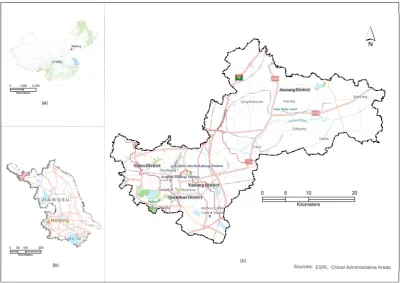
Xuzhou (33º43'-34º58'N, 116º22'-118º40'E) is located in the northwest of Jiangsu Province, China,
115
adjacent to Shandong, Henan, and Anhui provinces (Figure 1). There is about 300km away from Xuzhou
116
to Nanjing, Jinan, Zhengzhou and Hefei, the capitals of adjacent provinces. It is also the center city of
117
Huaihai Economic Zone, with the area of 17.6 million km2 and the population of 120 million. Xuzhou is
118
the largest city among the adjacent 19 cities, consisting of 5 administrative districts, 3 counties and 2
119
county-level cities. It is mostly comprised of plains, with small areas of hillocks and mountains in the
120
central and eastern regions. The Old Yellow River flows across the city generally in the west to southeast
121
direction, and the Yunlong Lake locates in the south of the region. For the purpose of this study, the
122
central area of the city was selected, which is composed of four districts, namely Quanshsn, Gulou,
123
Yunlong and Jiawang district. It covers an area of 1058 km2. During the three past decades, Xuzhou has
124
experienced significant economic growth and rapid urbanization. The urban population increased from
125
0.67 million in 1978 to approximately 2.02 million in 2015. The GDP has raised to 531.952 billion RMB
126
Yuan in 2015 against 2.14 billion in 1978 (Figure 2).
128
Figure 1. Map of China showing the location of Jiangsu province (Data Source: ESRI); (b) Map of Jiangsu
129
province showing the location of Xuzhou city center (Data Source: ESRI); and (c) Map of study area
130
131
Note: In 1993 and 2000, some administrative divisions were adjusted.
132
Figure 2. Population, built-up area and GDP growth of Xuzhou from 1978 to 2014 (Data Source:
133
2.2 Data and Preprocessing
135
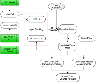
The analysis of land use changes and landscape pattern were conducted on the basis of
post-136
classification change detection strategy. The procedural workflow proposed in this study is illustrated in
137
Figure 3. Each component will be described in detail as follows, including data sources and
pre-138
processing, classification scheme, land use change and landscape pattern analysis.
139
140
Figure 3. Flowchart of the procedural workflow.
141
2.2.1 Landsat time series
142
With the free access to Landsat archive and other new remote sensing data sources online, it is
143
possible to exploit the multi-temporal remote sensing data to map urban changes. Google Earth Engine
144
is a cloud-based platform for planetary-scale environmental data analysis. It combines a petabyte-scale
145
archive of publicly available remotely sensed imagery and other data. Landsat series TOA Reflectance
146
data (Orthorectified) are involved in this study, including Landsat TM, ETM+ and Landsat OLI. They are
147
made from Level L1T orthorectified scenes, using the computed Top-of-Atmosphere (TOA) reflectance
148
[39]. These composites are created from all the scenes in each 32-day period beginning from the first day
149
of the year and continuing to the 352nd day of the year. The last composite of the year, beginning on day
150
353, will overlap the first composite of the following year by 20 days. All the images from each 32-day
151
period are included in the composite, with the most recent pixel as the composite value.
152
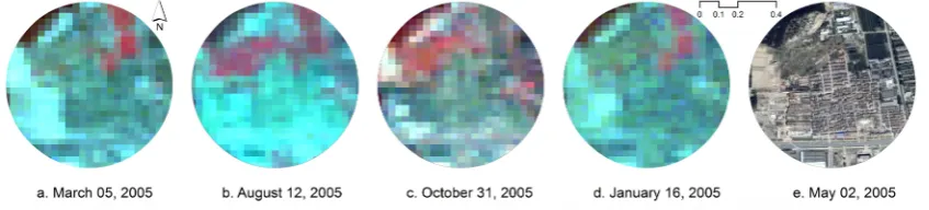
To avoid the confusion between new urban land and other land cover types (such as bare land,
153
follow or post-harvest cropland), it can be resolved combining images from multiple seasons (Figure 4).
There is often a high probability that bare or cropland will be vegetated during at least one season of each
155
year, and thus can be separated from built-up areas predominantly non-vegetated all the year round.
156
However, it is unrealistic to select all the seasonal imageries in a year.
157
158
Figure 4. Multispectral seasonal observations of built-up land and cropland from 30-m resolution Landsat
159
TM data in 2005 in a peri-urban area northwest of Xuzhou (the Near-infrared, Red and Green wavelengths
160
are set to R-G-B, a reference of the same area is shown in (e) from Google Earth).
161
Apart from the raw data or preprocessing data, Google Earth Engine also provide all kinds of
162
Composite product derived from raw data, such as 32-Day Composite for NDWI, NDVI, EVI. In this
163
study, we compared 32-Day NDVI Composite with the EVI Composite (Figure 5). For EVI, it is clear that
164
all the land use types have better separability, especially in summer (Figure 5). For Crop/Grass land, the
165
EVI has a high value than corresponding NDVI, the max value up to 1. Thus, the EVI was employed in
166
this study, which is generated from the Near-IR, Red and Blue bands of each scene, and ranges in value
167
from -1.0 to 1.0 [40] (Eq.(1)).
168
EVI = 2.5 × × . × (1)
169
Where 𝜌 , 𝜌 and 𝜌 are the top-of-atmosphere (TOA) reflectance of Blue, Red and NIR bands for
170
Landsat series imagery.
171
172
Figure 5. Comparison between the NDVI and EVI, derived from the Landsat 8 32-Day NDVI Composite
173
and EVI Composite in 2016
174
2.2.2 DMSP/OLS NTL data
175
The version 4 DMSP/OLS NTL data from the website of the National Geophysical Data Center at
176
the National Oceanic and Atmospheric Administration were also hosted on Google Earth Engine, which
177
is aggregated and composited to 30 arc second (about 1 km) grids
178
(https://ngdc.noaa.gov/eog/dmsp/downloadV4composites.html). It has a unique capability to detect
179
visible and near-infrared (VNIR) emission sources at night. Each image in the collection contains 4 bands,
180
i.e. avg_vis, cf_cvg, avg_lights_x_pct and stable_lights. The cleaned up avg_vis (stable_lights) was
181
selected in our study, which contains the lights from cities, towns, and other sites with persistent lighting,
182
including gas flares. Ephemeral events, such as fires have been discarded. The background noise was
183
identified and replaced with values of zero. The DN values of this band range from 0 to 63.
2.2.3 Data pre-processing
185
32-Day EVI Composites precede the NDVI Composites in distinguishing among the different land
186
use (Figure 5). Thus, 32-Day EVI Composites were involved in this study. Due to growth cycle and
187
seasonality of crop, it is difficult to determine the optimal TOA reflectance data for each year, which is
188
also affected by the clouds. Thus, in order to overcome the limitations, one effective approach is to
189
produce a maximum EVI image from multi-temporal EVI images. In this study, 32-Day EVI Composites
190
were selected for each year, which consist of 12 EVI images. For each pixel, we got the maximum of EVI
191
over the year and generated the EVImax imagery for each year. Another important role for the EVImax
192
imagery is to remove the impact of cloud contamination. Therefore, the final EVImax imagery is cloud-free
193
and has a data range between -1 and 1.
194
Due to the lack of on-board calibration and the difference between sensors, there are systematic
195
biases in NTL data. Consequently, the NTL data the individual composites had to be inter-calibrated
196
carefully to generate a consistent NTL time series [41-43]. Elvidge, Hsu, Baugh and Ghosh [43] . Pandey,
197
et al. [44] compared and evaluated existing nine calibration methods to provide guidance to us on their
198
relative strengths and weaknesses. This research results showed that inter-calibration reduces systematic
199
biases consistently across most countries using the methods adopted in [43] and [45]. Pandey, Zhang and
200
Seto [44], and suggests that Zhang, Pandey and Seto [45] can obtain marginally better results than
201
Elvidge, Hsu, Baugh and Ghosh [43].The coefficients for inter-calibration provided by Zhang, Pandey
202
and Seto [45] were adopted in our study.
203
While the calibrated DMSP/OLS NTL values are not recorded in the range [-1, 1], EVI values are
204
generated in the range [−1.0, 1.0]. To make them comparable, we normalize the calibrated DMSP/OLS
205
NTL into the range of [0.0, 1.0]. Then, we resample the normalized DMSP/OLS NTL data down to 30 m.
206
2.2.4 The Normalized Difference Enhanced Urban Index (NDEUI)
207
In recent years, DMSP/OLS NTL was widely used to study urban sprawl, and several
spectral
208
indices have been proposed.
Zhang, et al. [46] proposed a new index VANUI combining MODIS209
NDVI and DMSP/OLS NTL. Zhang, Li, Thau and Moore [28] proposed NDUI (Normalized Difference
210
Urban Index) combining ETM+ NDVI with normalized DMSP/OLS luminosity data to capture urban
211
spatial structures at a much finer scale. However, each annual NDVI composites was generated from
212
contiguous three-year ETM+ imageries, which will confuse changed land use types during the three
213
years, especially in the rapid development region. Furthermore, the thresholds of NDVI given by the
214
authors is nor suitable for all the cases. Cheng, et al. [47] constructed the BCI Assisted NTL Urban Index
215
(BANI) based on the correlations between BCI (Biophysical Composition Index) and normalized
216
DMSP/OLS NTL data. Here, the BCI was calculated using MODIS surface reflectance data, which not
217
only have several complex steps, including Tasseled Cap transformation but also only get the coarse
218
resolution BCI. Thus, in our study, we combine the EVImax imagery mentioned in section 2.3.1 with the
219
30m resolution normalized DMSP/OLS NTL data to generate a new index, i.e. NDEUI (Normalized
220
Difference Enhanced Urban Index) (Eq.(2)).
221
NDEUI = (NTL − EVI)/(NTL + EVI) (2)
222
Where NTL is the normalized DMSP-OLS stable nighttime lights data, and EVI is EVImax imagery
223
generated from the all the 32-Day EVI Composites for one year.
224
2.3 Classification with Random Forests
225
According to the definition given by Schneider and Mertes [48], urban land is dominated by the
226
built environment with more than 50% coverage ratio within a landscape unit, which include all
non-227
vegetative, human-constructed elements (building, roads etc.). Thus, five land cover categories were
classified from remote sensing imagery in this study, which are urban land, water bodies,
229
agriculture/grassland, forest and barren land.
230
The annual classification was implemented utilizing optimal Landsat TOA Reflectance as the base
231
scene and corresponding NDEUI. Due to the seasonal phenology of study area and cloud cover, a base
232
scene with less cloud cover acquired from July to October was preferred. It should be noted that there
233
are not DMSP/OLS NTL data before 1992 and after 2013. According to the Statistical Yearbook of Xuzhou
234
City, there is no obvious urban land change during the two periods. Thus, the DMSP/OLS NTL data was
235
replaced by the data of 1992 and 2013 in annual classification before 1992 and after 2013, respectively.
236
To reduce possible biases caused by training samples and get relatively classifiers, a hierarchical
237
sampling scheme [5] was adopted in our study. Firstly, with the support of EVImax imagery in 2005 and
238
Google Earth, training samples were collected on the cloud-based platform, i.e. Google Earth Engine.
239
Consequently, they were loaded as initial training samples of a specific temporally adjacent year, and
240
were rechecked to identify whether their types have been changed. We could reassign their types, move
241
to corresponding positions or delete for the changed samples. Thus, we repeated the procedure and
242
obtained all the training samples for all years.
243
Random Forests (RF) is an ensemble learning method for classification, regression and other tasks
244
[49], which uses trees as base classifiers. It is also considered as a combination of many classifiers and
245
conferred some special characteristics [50]. RF increases the diversity of the trees by making them grow
246
from different training data subsets created through bootstrap aggregating (bagging), which is a
247
technique used for training data creation by resampling the original dataset with replacement randomly
248
[51]. Several research results have shown that RF classifier performs better than other well-known
249
classifiers, because of its high efficiency, robustness to noise or outliers, high efficiency and lighter
250
computation [50, 52, 53]. In addition, it has the capability of a bigger number of variables and quantitative
251
measurement of variable contributions [5]. In theory, the RF classifier randomly selects a sample of the
252
training set and a sample of variables many times to generate a large number of small classification trees.
253
Then, all the small trees are aggregated to determine the final category by applying a majority vote rule
254
[49].
255
Two parameters should be defined in RF classifier for generating a prediction model, which are the
256
number of classification trees (k), and the number of prediction variables (m), used to split a RF node. In
257
general, the generalization error always is convergent and over-training is not a problem due to the
258
‘‘Strong Law of Large Numbers’’ with increasing the number of trees [51]. As well as, in order to make
259
each individual tree of the model to be less strong and reduce the correlation between trees, it is an
260
effective approach to reduce the number of predictive variables (m). Thus, it is essential to optimize the
261
parameters k and m to minimize the generalization error. In this study, based on the sensitivity
262
experiment, we applied the RF classifier with 500 classification trees. The number of prediction variables
263
(m) corresponds to the square root of the number of input variables [54]. The “Out-of-Bag” OOB accuracy
264
was employed to assess the performance of classification for each year, which is an unbiased estimator
265
of the classification OA accuracy and can be used to substitute the cross-validation [49]. Approximately
266
2/3 of the train data were used to train the classifier, while the remaining data to validate the training.
267
After classification, the mode filter (3*3) was used for post-classification procedures like
“salt-and-268
pepper” removal. Thus, the final LULC maps for 1985, 1995, 2005 and 2015 were generated (Figure 6).
270
Figure 6. LULC maps of Xuzhou city for (a) 1985, (b) 1995, (c) 2005 and (d) 2015 derived from Landsat
271
series imageries
272
2.4 Classification accuracy assessment
273
Accuracy assessment for individual classification is essential to correct and efficient analysis of
274
LULC change. A total number of 100 pixels checked using Google Earth and knowledge of the study area
275
for each class was collected on the basis of stratified random distribution method to conduct accuracy
276
assessment of each classification. The error matrix, overall accuracy and Kappa coefficient were
277
calculated for each classified land use maps and tabulated in Table 1 to Table 4, respectively. The overall
278
accuracies ranged from 97.8% to 98.8%, with Kappa coefficients from 0.9725 to 0.985.
279
Table 1 Accuracy assessment for the 1985 LULC map produced from Landsat TM.
280
Classified data
Reference data User's
Accuracy [%]
Kappa Accuracy
C1 C2 C3 C4 C5 Sum
Urban land (C1) 96 3 1 100 96 0.95 Agriculture/grass land (C2) 100 100 100 1
Water bodies (C3) 100 3 103 97.09 0.9636
Forest (C4) 94 94 100 1
Barren land (C5) 4 99 103 96.12 0.9515 Sum 100 100 100 100 100 500
Producer's Accuracy [%] 96 100 100 94 99 Overall Accuracy [%] 97.8
Kappa Coefficient 0.9725
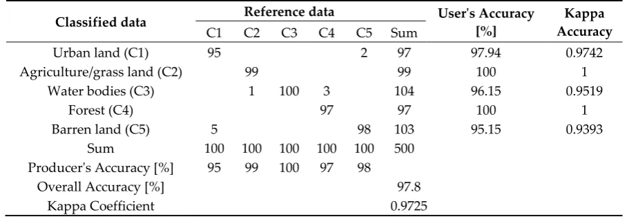
Table 2 Accuracy assessment for the 1995 LULC map produced from Landsat TM.
282
Classified data Reference data User's Accuracy
[%]
Kappa Accuracy
C1 C2 C3 C4 C5 Sum
Urban land (C1) 95 2 97 97.94 0.9742 Agriculture/grass land (C2) 99 99 100 1
Water bodies (C3) 1 100 3 104 96.15 0.9519 Forest (C4) 97 97 100 1 Barren land (C5) 5 98 103 95.15 0.9393
Sum 100 100 100 100 100 500 Producer's Accuracy [%] 95 99 100 97 98
Overall Accuracy [%] 97.8 Kappa Coefficient 0.9725
Table 3 Accuracy assessment for the 2005 LULC map produced from Landsat TM.
283
Classified data Reference data User's Accuracy
[%]
Kappa Accuracy
C1 C2 C3 C4 C5 Sum
Urban land (C1) 98 1 3 102 96.08 0.951 Agriculture/grass land (C2) 99 99 100 1
Water bodies (C3) 100 100 100 1 Forest (C4) 100 100 100 1 Barren land (C5) 2 97 99 97.98 0.9747
Sum 100 100 100 100 100 500 Producer's Accuracy [%] 98 99 100 100 97
Overall Accuracy [%] 98.8 Kappa Coefficient 0.985
Table 4 Accuracy assessment for the 2015 LULC map produced from Landsat OLI.
284
Classified data
Reference data User's Accuracy
[%]
Kappa Accuracy
C1 C2 C3 C4 C5 Sum
Urban land (C1) 100 2 5 107 93.46 0.9182 Agriculture/grass land (C2) 100 2 102 98.04 0.9755
Water bodies (C3) 100 100 100 1
Forest (C4) 98 98 100 1
Barren land (C5) 93 93 100 1 Sum 100 100 100 100 100 500
Producer's Accuracy [%] 100 100 100 98 93 Overall Accuracy [%] 98.2
Kappa Coefficient 0.9775
2.5 Land use change and landscape analysis
285
Land change analysis was carried out utilizing GIS-based spatial operations and landscape metrics
286
derived from the LULC maps. In this paper, we focus on the land use changes during the period of
1985-287
1995, 1995-2005, 2005-2015 and 1985-2015, especially on the growth of urban land and its spatial change
288
trend. Several qualitative and quantitative methods were employed to analyze the spatial landscape
289
patterns changes of land use at different stages. Here, landscape patterns were evaluated utilizing
landscape metrics, which can be calculated on the three deferent levels, namely patch-level, class-level
291
and landscape-level. In this study, class-level and landscape-level metrics were employed. Class-level
292
metrics are used to qualify the characteristics of the same LULC type and return a unique value for each
293
class in the landscape. On the other hand, landscape-level metrics return a unique value corresponding
294
to the landscape mosaic as a whole [55]. In order to reduce the correlativity, landscape metrics selected
295
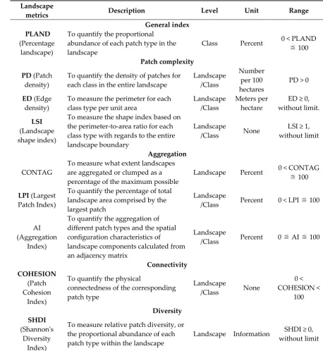
in this study are tableted in Table 5 [56].
296
Table 5 List and descriptions of landscape metrics used in this study
297
Landscape
metrics Description Level Unit Range
General index PLAND
(Percentage landscape)
To quantify the proportional abundance of each patch type in the landscape
Class Percent 0 < PLAND ≦ 100
Patch complexity
PD (Patch density)
To quantify the density of patches for each class in the entire landscape
Landscape /Class
Number per 100 hectares
PD > 0
ED (Edge density)
To measure the perimeter for each class type per unit area
Landscape /Class
Meters per hectare
ED ≥ 0, without limit.
LSI
(Landscape shape index)
To measure the shape index based on the perimeter-to-area ratio for each class type with regards to the entire landscape boundary
Landscape
/Class None
LSI ≥ 1, without limit
Aggregation
CONTAG
To measure what extent landscapes are aggregated or clumped as a percentage of the maximum possible
Landscape Percent 0 < CONTAG ≦ 100
LPI (Largest Patch Index)
To quantify the percentage of total landscape area comprised by the largest patch
Landscape
/Class Percent 0 < LPI ≦ 100
AI (Aggregation
Index)
To quantify the aggregation of different patch types and the spatial configuration characteristics of
landscape components calculated from an adjacency matrix
Landscape
/Class Percent 0 ≦ AI ≦ 100
Connectivity COHESION
(Patch Cohesion
Index)
To quantify the physical
connectedness of the corresponding patch type
Landscape
/Class None
0 < COHESION < 100 Diversity SHDI (Shannon's Diversity Index)
To measure relative patch diversity, or the proportional abundance of each patch type within the landscape
Landscape
metrics Description Level Unit Range
SIDI
(Simpson’s Diversity
Index)
To measure the probability that any two pixels selected at random would be different patch types
Landscape None 0 ≦ SIDI < 1
To visualize the spatiotemporal changes of landscape patterns and reveal their temporal and spatial
298
characteristics during the urbanization, the LULC maps of the four years were divided into 900m × 900m
299
grids using the gridsplitter plugin in QGIS, respectively. 1,424 subgrids were obtained in this study. The
300
landscape metrics at landscape level for each subgrid were calculated using the Fragstats 4.2 to analysis
301
spatiotemporal changes of landscape pattern.
302
3. Results and analysis
303
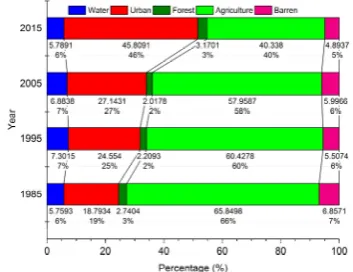
3.1 Change detection analysis
304
The changes detections were implemented for 1985-1995, 1995-2005, 2005-2015 and 1985-2015. Firstly,
305
we calculated the net area changes by category between the different years based on the LULC maps
306
(Figure 7). It is clear that urban land has significantly increased, while the agricultural land has been
307
drastically reduced. It is also can be seen from the PLAND (Percentage of Landscape) of different land
308
use in different years (Figure 8). During the period from 1985 to 1995, the urban area has increased by
309
6,082 ha that is more than 30.65%. In the next two decades, the urban area has increased by more than
310
10.54% and 68.78%, respectively (Figure 7, Figure 8, and Figure 9). It suggested a sharply ascending
311
trend in the development of the urban area, especially from 2005 to 2015.
312
Figure 9 present the gains and losses in urban area during the different period. On the contrary, the
313
agricultural land kept the peace of decrease and loosed 26,933 ha in the past 30 years. Overall, the urban
314
area has significantly increased by about 143.75% in the past three decades, at the main expense of
315
agricultural land in the study area. For the water bodies, there is an increase of 26.78%, which can be
316
explained by the subsidence result from coal mining from 1985 to1995. In the next two decades, the
317
government attached importance to the reclamation of subsidence, thus the water area has slightly
318
decreased by 5.72% and 15.90%, respectively. In general, it can be noted that there were no significant
319
changes in the area of water body. The forest increased the total number by 15.68%, while barren land
320
decreased by 28.63%. The transition mainly occurred from agricultural land to urban land from 1985 to
321
2015. Figure 10 illustrate the transition from other land use types to urban land in different periods.
322
323
Figure 7. Net area changes by category
324
between different years
325
326
Figure 8. Proportion of area for each class
327
329
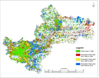
Figure 9. Maps presenting gains and losses in urban area during the period of (a) 1985-1995; (b)
1995-330
2005; (c) 2005-2015; and (d) 1985-2015.
331
332
Figure 10. Maps of land use transition from other land use types to urban land during the period of (a)
333
1985-1995; (b) 1995-2005; (c) 2005-2015; and (d) 1985-2015.
334
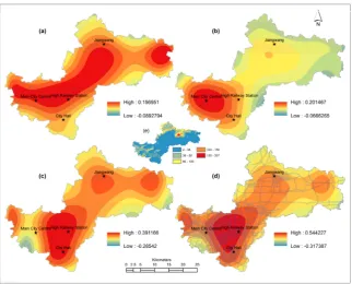
3.2 Spatial trend of changes
336
In landscapes dominated by human intervention, patterns of change can be complex, and thus very
337
difficult to decipher. Figure 11 shows the spatial sprawl of urban area in 1985, 1995, 2005 and 2015. To
338
reveal the spatial trend of urbanization, we created the spatial trend maps of changes from other lands
339
to urban land during the given periods adopting the 9th polynomial order, respectively (Figure 12).
340
As can be seen from the results, it is observed that continuous transition from other land use types
341
into urban land has appeared dual-core development throughout urbanization process, which are main
342
city region and Jiawang district, but with different development intensity in different periods. During
343
1985-1995, it is clear that there was a continuous increase in urban area between the two core regions
344
from southwest to northeast (Figure 12 (a)). In the subsequent 10 years, however, the expansion in the
345
urban area was mainly in all directions around the two core regions, especially in the main city region
346
(Figure 12 (b)). During the period of 2005-2015, it is a remarkable fact that the growth in the southeastern
347
part of the main city region was mainly due to the construction of new city region planned in 2004, which
348
is also the location of municipal government (Figure 12 (c)). By the end of 2015, the total investment was
349
up to about 70 billion yuan to construct the roads with the total length of about 110 km and 57 bridges,
350
as well as the residential growth of more than 5 million square meters (Report on the Work of Xuzhou
351
Municipal Government in 2016). As also can be seen in Figure 12(c), the high railway station available in
352
2011 gave the contribution to the growth of urban area. Overall, in the past three decades, the continuous
353
increase in the urban area was mainly occurred between the new city region and the Jiawang district,
354
mainly affected by construction of new city region, freeway and the high railway station (Figure 12 (d)).
355
Compared with DEM (Figure 12(e)), terrain is also one of the factors, affecting the spatial trend of urban
356
area changes. In the southwest and northeast of the study area, the topography undulated greatly and
357
the degree of urbanization was lower than that of other areas.
358
359
361
Figure 12. Spatial trend of urban growth during given periods: (a) from 1985-1995; (b) from 1995-2005; (c)
362
from 2005-2015; (d) from 1985-2015, and (e) DEM of study area.
363
3.3 Changes analysis of landscape metrics
364
As shown in Figure 8 and Figure 10, the transition of land use types occurred mainly from
365
agricultural land to urban land from 1985 to 2015. Thus, the changes and relationships measured based
366
on different landscape metrics at the class level were analyzed between urban land and agricultural land.
367
Here, the landscape metrics can be fit into four major categories to represent different aspects of the
368
landscape pattern: Patch complexity (represented by PD, ED and LSI), aggregation (represented by LPI
369
and AI), connectivity (represented by COHESION) and diversity (represented by SHDI and SIDI) (Table
370
5).
371
As can be seen from Figure 13, all the landscape metrics of urban land and agricultural land have
372
undergone tremendous changes during the study period. In terms of PD, urban land use was on a
373
downward trend while agricultural land use was continuously increasing (Figure 13 (a)). On the
374
contrary, there was the consistent trend of changes in ED of agricultural land and urban land, reaching
375
their lowest values in 2005, then dramatically increasing up to 48.853m/ha and 55.9287m/ha in 2015,
376
respectively (Figure 13 (b)). Considering urban land, the date on LSI are interesting, the value decreased
377
rapidly from 75.4532 in 1985 to 58.1453 in 2005, but then increasing again up to 68.1731 in 2015. The LSI
378
of agricultural land appeared an overall increase from 41.6725 in 1985 to 64.2222 in 2015, except for a
379
slight decrease in 2005 (Figure 13 (c)).
380
Figure 13 (d) illustrates that with significant decreasing in LPI of agricultural land, the LPI of urban
381
Continued to increase, with an increase of more than 18.5%. Meanwhile, there was a gradual increase in
382
AI of urban land, reaching 90.8229% in 2015. In term of agricultural land, however, it gradually dropped
383
from 95.3672% in 1985 to 90.7922% in 2015 (Figure 13 (e)). Obviously, the aggregation of urban land
384
gradually increased and surpassed that of agricultural land during the process of the past three-decade
385
urbanization. With regard to COHESION, the values of agricultural land changed from 99.8371 to
386
99.0596, and urban land from 97.7713 to 99.6485 during the study period.
388
Figure 13. Line diagrams illustrating the changes and relationships of landscape metrics between the
389
urban land and agriculture land at the class level.
390
Figure 14 shows the landscape-level metrics changes during the period of 1985-2015. The
391
descriptions of landscape metrics used are tabulated in Table 5. As we can see from Figure 14(a to c), 2005
392
had the lowest patch complexity, increasing to their maximums in 2015. There is no doubt that the highest
393
rates of change in the three metrics were observed in the period between 2005 and 2015. In terms of
394
urbanization modes, this may indicate that infilling and edge-expansion modes were dominant in
395
Xuzhou city before 2005, and then leapfrog mode. LPI declined from 30.2737% in 1985 to 13.9131% in2005,
396
which may be the evidence that the agricultural land was dominant in 1985. However, it increased again
397
to 23.9468% in 2015 (Figure 14 (d)). Combined with change detection discussed in 3.1, it could be
398
concluded that the dominant land use type was shifted from agricultural land to urban land. It is clear
399
from the Figure 14 that the CONTAG and AI metrics were considered to be inversely related to LSI. They
400
tend to slightly fluctuate, but then dramatically decreased from the year 2005. This tendency affirmed
401
that landscape pattern was vastly disaggregated and less contiguous pattern in 2015, mainly owing to
402
continued increasing leapfrog urban land.
403
Figure 14 (g) shows the changes of the COHESION. The COHESION value decreased sharply,
404
reaching its lowest value of 99.2116 in the year 1995. Thereafter it increased continuously in the late stage
405
of urbanization.
406
Both SHDI and SIDI measure relative diversity. From 1985 to 2015 the two diversity metrics
407
increased constantly (Figure 14 (h, i)), indicating an increasing heterogeneity in this landscape. This fact
408
is already evident that agriculture became segmented into smaller patches as the continual increase in
409
urban land.
411
Figure 14. Line graph depicting the landscape-level metrics changes from 1985 to 2015
412
3.4 Spatiotemporal changes analysis of landscape pattern
413
At the landscape level, Landscape metrics calculated on the basis of subgrids well depict landscape
414
pattern characteristics of each subgrid and contribute to revealing the spatiotemporal change of the study
415
area. Furthermore, from the spatiotemporal changes of the landscape pattern, urban core, urban fringe,
416
and rural area can be well discerned. Here, we mapped the spatial distribution of each landscape metric
417
for different years utilizing the quantile grading method (Figure 15). It is clear that the landscape patterns
418
have changed remarkably in the process of urbanization in Xuzhou City.
419
For the PD Landscape metric, urban core and rural areas are associated with lower values, which
420
are mainly dominated by urban land and agricultural land, respectively, while urban fringe areas are
421
opposite. From the perspective of spatiotemporal changes, the urban core area was expanding
422
continuously, while the PD landscape metric in rural areas continued to increase, indicating that
423
agricultural land was continuously transited into urban land and appear a tendency of fragmentation in
424
the process of urbanization. AI, however, is opposite to PD, with higher values in urban core and rural
425
areas and lower values in urban fringes. As can be seen from Figure 15, ED and PD have a similar
426
spatiotemporal change tendency. During the process of urbanization, the values surrounding the urban
427
core area had a slight decrease, which marked that the core area continued to expand. From the southeast
428
to the northeast of the main urban region, however, the value has been obviously increasing, especially
429
in 2015, mainly due to the construction of new city region and the high railway station resulting in a large
430
amount of transition from agricultural land into urban land. As LPI is used to quantify the percentage of
431
total landscape area comprised of the largest patch, it is a simple measure of dominance. For instance,
432
LPI map (a) in Figure 15 gives prominence to old city region and distribution of agricultural land. With
433
the fragmentation of agricultural land, LPI map (d) clearly highlight the urban core area. The COHESION
434
maps reveal connectivity of the patches in the study area and represent the impact extent of urban
435
expansion. Compared with COHESION map (a) in Figure 15, COHESION map (d) has obviously
436
decreased in the southeast of the main city region, which just verifies the vigorous development of the
new city region in recent years. Regarding SHDI, although there was a marked decrease in 2005, SHDI
438
showed a significant increase trend, mainly due to the continuous expansion of the urban area and the
439
promotion of a large number of municipal projects in recent years, including the construction of the
440
freeways and the subways. Taking into account the evolution of urban, all landscape metrics used in this
441
study were mutually corroborated in terms of spatiotemporal characteristics. The changes at
landscape-442
level metrics in subgrids effectively reveal the spatiotemporal evolution process of urbanization during
443
the study period.
Figure 15. Spatiotemporal changes of landscape metrics: (a) 1985, (b) 1995, (c) 2005 and (d) 2015
445
4. Discussion
446
4.1 NDEUI as an effective index for improving the classification accuracy
447
An index NDEUI was proposed in this study, combined with annual maximum EVI and
448
corresponding DMSP/OLS NTL, which effectively reduce confusion between urban areas and barren
449
land, as well as fallows. The advantage owes to the fact that annual maximum EVI makes sure the
450
agricultural lands have maximum EVI values obtained in growing seasons to decrease the impact from
451
seasonal fallow lands. Furthermore, since barren lands, especially far away from urban area, are
452
associated with extremely low value in NTL, DMSP/OLS NTL can effectively separate them from urban
453
lands. It is necessary that 1-km resolution normalized NTL data downscale in the size of 30 m. Firstly,
454
we generated annual maximum EVI from 32-Day EVI Composites for each year. Secondly, the NDEUI
455
for each year was calculated. Afterwards, a new composite was generated combing with NTL, annual
456
maximum EVI and Landsat raw bands, and used to obtain the land use classification by means of
457
Random Forests classifier. In this study, all the procedures were implemented on a free cloud computing
458
platform, namely Google Earth Engine. The GEE, based on its cloud-computing and storage capability,
459
has archived a large number catalog of earth observation data and enabled researchers to work on the
460
trillions of images online. It represents one of the most powerful tools up to now in remote sensing with
461
its ability to analyze and classify remotely sensed data over different temporal scales. In this study, the
462
GEE provided us an effective approach to obtain the land cover classifications by JavaScript.
463
4.2 Relationship of urbanization and changes dynamic of landscape pattern
464
Analysis the changes in landscape metrics contribute to demonstrate the urban growth modes in the
465
different process of urbanization. Usually, there are three urban growth modes discussed in previous
466
literature, i.e. infilling, edge-expansion and leapfrog mode [35, 57, 58]. In this study, several landscape
467
metrics at class/landscape level depicted in detail in Section 3 were selected to characterize their
468
spatiotemporal changes, generating a large quantity of information on landscape patterns. All the
469
information could determine which urban growth mode was dominant, as well as indicate the degree
470
affected by urbanization at different stage during the study period. The gradual changes in landscape
471
metrics imply that the landscape was undergoing a major transformation from one dominant land cover
472
to another resulting from urbanization. On the other hand, this dramatic land cover change caused by
473
rapid urbanization has resulted in an essential change of landscape patterns. It could be clear that there
474
are some inherent relationships between the process of urbanization and the changes in landscape
475
metrics no matter at class or landscape level. Consequently, it is effective and feasible to study the
476
urbanization utilizing landscape metric.
477
Considering the urban growth modes, the analysis based on the results are as follow. With a slight
478
increase of infilling area, urban growth mainly occurred as leapfrog mode along both sides of the roads
479
during the period of 1985-1995, resulting in a slightly decreased aggregation of the landscape.
480
Subsequently, the urban growth mode shifted into expansion. With the increasing of
edge-481
expansion growth in urban area, the urban land has become more aggregated and compact at this stage,
482
especially in the main city region, reflected by the decreasing PD, ED and LSI as well as the increasing
483
AI. Since 2005, the process of urbanization was accelerated, and urban growth mainly appeared from the
484
southeast to the northeast of the main city region, owing to the construction of new city region and other
485
infrastructures. At this stage, the edge-expansion and leapfrog modes coexisted, causing different change
486
degree of landscape metrics in different region. All the urbanization processes in different stages are
487
reflected in spatiotemporal changes of landscape metrics.
5. Conclusion
491
Urbanization is an irreversible process, and rapid urbanization has resulted in drastic changes in
492
LULC and landscape patterns over the past three decades, particularly in the developing countries.
493
Mapping and monitoring of LULC change, therefore, are crucial to generating information for
494
policymakers and planners, as well as helping to understand the underlying socio-economic and
495
biophysical processes in urban areas. Accordingly, a GIS&RS-based integrated approach was used to
496
quantitatively characterize the land use/land cover pattern and dynamics of urban sprawl in Xuzhou city
497
during the period of 1985–2015.
498
In this study, we integrated NTL with annual maximum EVI and proposed a new spectral index,
499
namely NDEUI. NDEUI-assisted Random Forests algorithm was implemented to obtain the LULC maps
500
in 1985, 1995, 2005 and 2015, respectively. The results indicate that the classification scheme proposed
501
achieved higher accuracy, reducing confusion between urban areas and barren land, as well as fallows.
502
The results show that Xuzhou city has experienced rapid urbanization over the past three decades. Urban
503
areas have increased by 143.75%, covering approximate 2.44 times the urban area in 1985, resulting in a
504
considerable decrease in agricultural land. Among the three decades, the highest growth in urban land
505
is up to 68.78% from 2005 to 2015, averaging nearly 7% per year. As can be seen from the analysis of the
506
urban growth spatial trend that the urban growth is proceeding in different directions during the
507
different period. Overall, the urban growth has appeared dual-core development mode throughout the
508
urbanization process. the process of urbanization in the north-east direction of the main city region,
509
mostly appears growth of Industrial area in the first two decades, whereas, in the southeastern direction,
510
the urban growth is mostly due to due to the construction of new city region planned in 2004 and the
511
high railway station available in 2011, as well as accompanied the growth of residential area. It should
512
be noted that the terrain and roads are also important factors affecting urbanization.
513
Statistical analysis may have a limited power to demonstrate the inherent relationship between
514
LULC changes, accordingly the dynamic changes of landscape pattern affected by urbanization were
515
studied. Six landscape metrics at the class level were calculated to reveal the dynamic changes of
516
landscape pattern in urban land and agricultural land. The changes in selected landscape metrics indicate
517
a lower aggregation and connectivity in agricultural land due to increasing dominance of urban land
518
during the study period. On the other hand, nine landscape metrics were also calculated to indicate the
519
landscape metrics changes at the landscape level. The landscape-level metrics changes suggest that there
520
appeared an increasing spatial heterogeneity along with the process of rapid urbanization during the
521
period of 1985-2015. Furthermore, to visualize the spatiotemporal changes of landscape patterns and
522
reveal their temporal and spatial characteristics during the urbanization, we divided all the LULC maps
523
into subgrids with the size of 900 m×900 m and calculated their landscape metrics at the landscape level.
524
The findings suggest that different urbanization modes and intensity result in variously the
525
spatiotemporal evolution of landscape patterns. In terms of urban growth mode, it can be concluded
526
from the above analysis that the urban growth mainly appeared a leapfrog mode alone both sides of the
527
roads during the period of 1985 to 1995, and then shifted into edge-expansion mode during the period
528
from 1995 to 2005, whereas the edge-expansion and leapfrog modes coexisted for the period from 2005
529
to 2015, causing different change degree of landscape metrics in different region. Overall, the high
530
valuable spatiotemporal information generated utilizing RS and GIS may give assistance to urban
531
planners and policymakers to well understand urban dynamics and evaluate their spatiotemporal and
532
environmental impacts at a local level for the sake of sustainable urban planning in the future.
533
534
Acknowledgments: We would like to express our respects and gratitude to the anonymous reviewers and editors
535
for their professional comments and suggestions on improving the quality of this paper. This work was supported
536
by the Visiting Research Scholar Program of the China Scholarship Council (Grant No. 201606425072), A Project
537
References
539
1. Zhang, J.; Li, P. J.; Wang, J. F., Urban Built-Up Area Extraction from Landsat TM/ETM plus Images Using
540
Spectral Information and Multivariate Texture. Remote Sensing 2014, 6, (8), 7339-7359.
541
2. Reynolds, R.; Liang, L.; Li, X. C.; Dennis, J., Monitoring Annual Urban Changes in a Rapidly Growing Portion
542
of Northwest Arkansas with a 20-Year Landsat Record. Remote Sensing 2017, 9, (1), 71.
543
3. Verhasselt, Y., Urbanization and Health in the Developing World. Soc Sci Med 1985, 21, (5), 483-483.
544
4. Minshull, R., Urbanisation: Changing environments. Geography 1998, 83, (360), 297-297.
545
5. Li, X.; Gong, P.; Liang, L., A 30-year (1984–2013) record of annual urban dynamics of Beijing City derived
546
from Landsat data. Remote Sensing of Environment 2015, 166, 78-90.
547
6. Li, X. C.; Liu, X. P.; Gong, P., Integrating ensemble-urban cellular automata model with an uncertainty
548
map to improve the performance of a single model. Int J Geogr Inf Sci 2015, 29, (5), 762-785.
549
7. Zhang, P.; Imhoff, M. L.; Bounoua, L.; Wolfe, R. E., Exploring the influence of impervious surface density
550
and shape on urban heat islands in the northeast United States using MODIS and Landsat. Can J Remote
551
Sens 2012, 38, (4), 441-451.
552
8. Ceplova, N.; Kalusova, V.; Lososova, Z., Effects of settlement size, urban heat island and habitat type on
553
urban plant biodiversity. Landscape and Urban Planning 2017, 159, 15-22.
554
9. Schneider, A., Monitoring land cover change in urban and pen-urban areas using dense time stacks of
555
Landsat satellite data and a data mining approach. Remote Sensing of Environment 2012, 124, 689-704.
556
10. Lu, M.; Chen, J.; Tang, H. J.; Rao, Y. H.; Yang, P.; Wu, W. B., Land cover change detection by integrating
557
object-based data blending model of Landsat and MODIS. Remote Sensing of Environment 2016, 184,
558
374-386.
559
11. Coulter, L. L.; Stow, D. A.; Tsai, Y. H.; Ibanez, N.; Shih, H. C.; Kerr, A.; Benza, M.; Weeks, J. R.; Mensah, F.,
560
Classification and assessment of land cover and land use change in southern Ghana using dense stacks of
561
Landsat 7 ETM + imagery. Remote Sensing of Environment 2016, 184, 396-409.
562
12. Yang, Y. T.; Wong, L. N. Y.; Chen, C.; Chen, T., Using multitemporal Landsat imagery to monitor and model
563
the influences of landscape pattern on urban expansion in a metropolitan region. J Appl Remote Sens
564
2014, 8, (1), 083639.
565
13. Mihai, B.; Nistor, C.; Simion, G., Post-socialist urban growth of Bucharest, Romania – a change detection
566
analysis on Landsat imagery (1984–2010). Acta geographica Slovenica 2015, 55, (2), 223-234.
567
14. Schneider, A.; Friedl, M. A.; Potere, D., A new map of global urban extent from MODIS satellite data.
568
Environ Res Lett 2009, 4, (4).
569
15. Xian, G.; Homer, C.; Demitz, J.; Fry, J.; Hossain, N.; Wickham, J., Change of Impervious Surface Area
570
Between 2001 and 2006 in the Conterminous United States. Photogramm Eng Rem S 2011, 77, (8),
758-571
762.
572
16. Gong, P.; Wang, J.; Yu, L.; Zhao, Y. C.; Zhao, Y. Y.; Liang, L.; Niu, Z. G.; Huang, X. M.; Fu, H. H.; Liu, S.; Li, C.
573
C.; Li, X. Y.; Fu, W.; Liu, C. X.; Xu, Y.; Wang, X. Y.; Cheng, Q.; Hu, L. Y.; Yao, W. B.; Zhang, H.; Zhu, P.; Zhao,
574
Z. Y.; Zhang, H. Y.; Zheng, Y. M.; Ji, L. Y.; Zhang, Y. W.; Chen, H.; Yan, A.; Guo, J. H.; Yu, L.; Wang, L.; Liu, X.
575
J.; Shi, T. T.; Zhu, M. H.; Chen, Y. L.; Yang, G. W.; Tang, P.; Xu, B.; Giri, C.; Clinton, N.; Zhu, Z. L.; Chen, J.;
576
Chen, J., Finer resolution observation and monitoring of global land cover: first mapping results with
577
Landsat TM and ETM+ data. Int J Remote Sens 2013, 34, (7), 2607-2654.
578
17. Selkowitz, D. J.; Stehman, S. V., Thematic accuracy of the National Land Cover Database (NLCD) 2001 land
579
cover for Alaska. Remote Sensing of Environment 2011, 115, (6), 1401-1407.
580
18. Han, R.; Li, Z. L.; Ti, P.; Xu, Z., Experimental Evaluation of the Usability of Cartogram for Representation of
581
GlobeLand30 Data. Isprs Int J Geo-Inf 2017, 6, (6).
582
19. Liang, D.; Zuo, Y.; Huang, L. S.; Zhao, J. L.; Teng, L.; Yang, F., Evaluation of the Consistency of MODIS Land
583
Cover Product (MCD12Q1) Based on Chinese 30 m GlobeLand30 Datasets: A Case Study in Anhui
584
Province, China. Isprs Int J Geo-Inf 2015, 4, (4), 2519-2541.
585
20. Li, G.; Lu, D.; Moran, E.; Hetrick, S., Mapping impervious surface area in the Brazilian Amazon using
586
Landsat Imagery. Gisci Remote Sens 2013, 50, (2), 172-183.
587
21. Lu, D. S.; Weng, Q. H., Spectral mixture analysis of the urban landscape in Indianapolis with landsat ETM
588
plus imagery. Photogramm Eng Rem S 2004, 70, (9), 1053-1062.
589
22. Boldt, M.; Thiele, A.; Schulz, K., Object-based Urban Change Detection Analyzing High Resolution Optical
590
Satellite Images. Earth Resources and Environmental Remote Sensing/Gis Applications Iii 2012, 8538.