Progress in the Global Modeling of the Galactic Magnetic Field
MichaelUnger1,∗and GlennysFarrar2,∗∗
1Institute for Nuclear Physics, Karlsruhe Institute of Technology, Karlsruhe, Germany 2Center for Cosmology and Particle Physics, New York University, New York, USA
Abstract.We discuss the global modeling of the properties of the Galactic Magnetic Field (GMF). Several improvements and variations of the model of the GMF from Jansson & Farrar (2012) (JF12) are investigated in an analysis constrained by all-sky rotation measures of extragalactic sources and polarized and unpolarized synchrotron emission data from WMAP and Planck. We present the impact of the investigated model variations on the propagation of ultrahigh-energy cosmic rays in the Galaxy.
1 Introduction
Magnetic fields are a major constituent of the interstellar medium of galaxies. Their energy density in the Galac-tic plane is about 0.6 eV/cm3 for a typical total magnetic field strength of 5µG and thus comparable to the energy density of cosmic rays (0.8-1.0 eV/cm3[1]) and interstel-lar radiation fields (star light and CMB, each contributing about 0.25 eV/cm3). The Galactic magnetic field (GMF) plays therefore an important role for the transport and en-ergy loss of Galactic cosmic rays. Furthermore, it is a ma-jor nuisance for the study of the origin of ultrahigh-energy cosmic rays as it deflects the arrival directions of extra-galactic charged particles on their way through the Galaxy to Earth. The origin of the large-scale GMF is still not fully understood, but it is widely assumed that it is pro-duced by the transfer of mechanical into magnetic energy via the dynamo mechanism (see e.g. [2]).
Different observational tracers of the GMF are sum-marized in [3]. In the following we focus on
(a) Multi-frequency observations of the Faraday rotation of extragalactic radio sources. The corresponding rota-tion measures (RMs) are proportional to the integral of the magnetic field parallel to the line of sight weighted with the density of thermal electrons of the warm ionized medium of the Galaxy.
(b) Measurements of the polarized synchrotron emission of cosmic-ray electrons. The total polarized intensity (PI) is proportional to the integral of the ordered component of the magnetic field perpendicular to the line of sight and weighted by the density of cosmic-ray electrons. The di-rection of the transverse magnetic field component can be inferred from the Stokes parameters Q and U.
(c) Measurements of the total (polarized and unpolarized) synchrotron intensity I, which gives a measure of the line-of-sight integral of the product of cosmic-ray electron
den-∗[email protected] ∗∗[email protected]
sity and total magnetic field strength (perpendicular coher-ent field and unordered, random magnetic field).
The most complete attempt to determine the global structure of the Galactic magnetic field (GMF) from these observations is the model of Jansson & Farrar [4, 5] (JF12). In this model, the GMF is described by a superpo-sition of three divergence-free large-scale regular compo-nents: a spiral disk field, a toroidal halo field and a poloidal field (“X-field”). In addition, there is a turbulent field model whose disk component is following the same spi-ral structure as the regular component and whose extended halo field strength is modeled as a Gaussian in height from the Galactic disk and as an exponential in Galactic radius. Account is taken of the possibility of the turbulent field having a preferred direction through a striation parameter. The parameters of the model are derived by minimizing theχ2between synthetic sky maps of RM, Q, U and I and the observations.
In the following we will describe our ongoing work to improve the JF12 model and to study uncertainties in determination of its parameters. Further information about the model fitting and calculation of simulated sky maps can be found in [6].
2 Variations and Improvements of the
JF12 Model of the Large-Scale GMF
2.1 Smooth Spiral Field
x [kpc] 15
− −10 −5 0 5 10 15
y [kpc]
15
−
10
−
5
−
0 5 10 15
5
−
4
−
3
−
2
−
1
−
0 1 2 3 4 5
B
/
µ
G
x [kpc] 15
− −10 −5 0 5 10 15
y [kpc]
15
−
10
−
5
−
0 5 10 15
5
−
4
−
3
−
2
−
1
−
0 1 2 3 4 5
B
/
µ
G
x [kpc] 15
− −10 −5 0 5 10 15
y [kpc]
15
−
10
−
5
−
0 5 10 15
5
−
4
−
3
−
2
−
1
−
0 1 2 3 4 5
B
/
µ
G
Figure 1.Fits of the coherent disk field. Upper Left:
“Wedge”-model of Brown+07 with fixed pitch angle ofα = 11.5◦
. Up-per Right: Smooth model with three modes (α=(13.4±0.7)◦
). Lower Middle: Smooth model with four modes (α=(14±0.5)◦
). The Sun is located atx=−8.5 kpc andy =0 kpc and the mag-netic field strength is shown in color.
magnetic field strength at reference radiusr0 into modes miwith phaseφ∗i:
B(r0)=
n X
i=1
Bicos mi(φ0−φ∗i)
(1)
with which the magnetic field at (r, φ) is given by
B(r, φ)=(sinα,cosα,0) r0
r B(r0). (2)
A spiral with three modes (upper right panel of Fig.1) im-proves the fit quality with respect to the baseline model with a discontinuous spiral by∆χ2 = 166 (the baseline model has χ2/ndf = 7292/6585). Four modes yields an additional improvement of∆χ2 = 18 (lower panel of Fig.1). Adding more modes does not improve the fit sig-nificantly. The pitch angle of the logarithmic spiral is a free parameter of the fit and we obtainα= (13.4±0.7)◦ and (14 ±0.5)◦ for n = 3 and 4 respectively, i.e. the pitch angle of the magnetic field is similar to but not the same as that of other probes of the spiral arms (see e.g. [8]) in accordance of observations of magnetic fields in nearby galaxies [9]. Further refinements of the JF12 spi-ral model are underway taking also into account rotation measures from Galactic pulsars with known distances (see also [10,11]).
2.2 Flaring Disk Field
Observations of the distribution of Hi, CO and stars are
compatible with an exponential increase of the vertical scale heighth of the Galactic disk [12], with increasing distance from the Galactic center:
h(r)=h0erhr (3)
x [kpc] 20
− −15 −10 −5 0 5 10 15 20
z [kpc]
1
−
0.8
−0.6 −0.4 −0.2
− 0
0.2 0.4 0.6 0.8 1
B [a.u.]
2
−
10
1
−
10 1
Figure 2. Side view of a exponentially flaring radial disk field
(h0=0.13 kpc andrh=9.22 kpc).
withh0 =0.13 kpc andrh =9.22 kpc for Hi[13].
Adopt-ing the same behavior for the vertical scale height of the disk field induces a vertical component:
Bz(r, φ,z)=Br(r, φ,z)
z rh
. (4)
An illustration of a flaring radial disk field (Br(r, φ,z) 1/r) is shown in Fig. 2. Applying the
flaring to the JF12 model with a freely floating radial scale rhconverges to very large values ofrh, i.e. our preliminary
conclusion is that the data does not support a strong flaring of the magnetic disk field, but further studies are needed for a definite conclusion.
2.3 Galactic Warp
It is well known that the Galaxy disk is not perfectly pla-nar but considerably warped, possibly caused by the grav-itational pull of the Magellanic clouds on the Milky Way. Adding the Galactic warp from [14] to our model, changes the fit quality by only∆χ2 = 8, and therefore it can be concluded that the current data is not very sensitive to the warp. However, the warp changes the low-latitude mag-netic field towards the outer Galaxy and is therefore im-portant for the backtracking of UHECRs in this direction.
2.4 Twisted X-Field
As noted in [16], the directions of the toroidal halo com-ponents derived in the JF12 model (in the same direction as the Galaxy’s rotation in the south and opposite to it the north) are the directions which would result from diff eren-tial rotation of the poloidal component. In the JF12 model the toroidal and poloidal components were fitted indepen-dently, but if indeed the toroidal component is produced from the poloidal by differential rotation, there is a more detailed relationship between the radial and vertical be-havior of their field strengths.
Consider an X-field that is dragged along with the ro-tation of the Galaxy. The MHD evolution of a magnetic field is [17]
∂tB=∇ ×(v×B)− ∇ ×η(∇ ×B)
| {z } =0 forσ→∞
(5)
where the “frozen-in condition” applies for infinite con-ductivity (magnetic diffusivityη→0 whenσ→ ∞). Un-der these conditions and for a purely azimuthal rotation
∂tB=∇ ×(v×B)=
−vr∂φBr ∂z(vBz)+∂r(vBr)
−vr∂φBz
15
− −10−5 0 5 10 15
x [kpc]
15 − 10 − 5 − 0 5 10 15
y [kpc]
4 −
3 −
2 −
1 −
0 1 2 3 4
z [kpc]
15
− −10−5 0 5 10 15
x [kpc]
15 − 10 − 5 − 0 5 10 15
y [kpc]
4 −
3 −
2 −
1 −
0 1 2 3 4
z [kpc]
15
− −10−5 0 5 10 15
x [kpc]
15 − 10 − 5 − 0 5 10 15
y [kpc]
4 −
3 −
2 −
1 −
0 1 2 3 4
z [kpc]
15
− −10−5 0 5 10 15
x [kpc]
15 − 10 − 5 − 0 5 10 15
y [kpc]
4 −
3 −
2 −
1 −
0 1 2 3 4
z [kpc]
r [kpc]
0 2 4 6 8 10 12 14 16
[km/s]φ
v
0 50 100 150 200 250 300
HMSFRs fit
(a) t=0 Myr (b) t=70 Myr (c) data
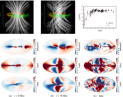
Figure 3. Illustration of the GMF model with a twisted poloidal field. The best-fit model att=70 Myr is presented in the middle
column and the corresponding un-twisted model att=0 is shown in the left column. The lower three rows show the simulated sky maps for RM, Q and U. A visualization of field lines of the models is in the top row. The lines are colored if the toroidal field strength is≥99% of the total field strength. Regions withr·B>0 are shown in orange, otherwise green is used. The observed sky maps are displayed in the lower three panels of the right-most column (Q and U data from [15], RM data compilation from [4] (see references therein)).. he rotation curve of the Galaxy used for the twisting is shown as a red line in the top-right panel together with measured velocities of high-mass starforming regions (HMSFRs) from [8].
Thus for a magnetic field that is poloidal and azimuthally symmetric att=0,Bφ(only) evolves with time:
Bφ(t)=(Bz∂zv+rBr∂rω)t, (7)
where we introduced the angular velocityω=ωeφ= vreφ and used the solenoidality of the poloidal field.
Eq. (7) can be applied to evolve any type of poloidal field. For definiteness, we tested this ansatz by evolving the smooth poloidal field model of type “C” from [18]. For the Galactic rotation curve we used a fit to the high-mass starforming regions with parallax measurements from [8] (see top right panel of Fig.3) and for the vertical velocity gradient we assume a constant value inspired by simula-tions [19] and constrain it within two sigma of the value of (22±6) (km/s)/kpc as observed close to the Galactic mid-plane [20]. The resulting sky maps of RM, Q and U of the un-twisted model and the evolved model (t=70 Myr) are shown in the left and middle panel of Fig.3. In contrast to the conclusions of [21], we find a good description of the overall structure of data from the combined effect of
radial and vertical shear, in particular the anti-symmetric pattern of the rotation measures and the tilted pattern of Q and U within the Solar circle. (The analytics underlying the contrary conclusion of [21] are not apparent to us.) In a future work we will discuss the magnitude and physical origin of the effective winding time≈70 Myr.
2.5 Thermal Electron Model
A large-scale model of the density of thermal electrons in the Galaxy (ne) is needed to predict the rotation
mea-sures for a given magnetic field configuration. The spatial distribution ofnecan be estimated using dispersion
but the more important difference between the two models is their particular parametric choices for the model compo-nents, such as for instance the thickness and pitch angles of the spiral arms. Both models give a similar good de-scription of the observed dispersion measures of pulsars. The main difference between the models for inferring the magnetic fields is the different electron density in the halo. A larger magnetic field strength in the halo is inferred us-ing YMW17 due to the lower density of electrons at large Galactic height in this model. The fitted field strengths for the toroidal and poloidal components are about a factor two larger than if derived using NE2001.
In addition to studying the influence of the warm ionized medium on the GMF modeling, we also tested the effect of adding the large-scale hot ionized medium from [25] to the calculation of RMs. No significant change of the inferred GMF was found in this case.
2.6 Correlation ofneandB
In the baseline fit for the parameters of the GMF the mag-netic field and thermal electron density are taken to be un-correlated. However, as pointed out in [26], pressure equi-librium between the ISM plasma and the magnetic field can lead to an anti-correlation between the two quanti-ties, leading to an underestimation of the magnetic field inferred from RMs. By contrast, compression leads to an enhancement of both magnetic field and gas density and results in a positive correlation of the two quantities, leading to an overestimation of the magnetic field inferred from RMs if this is not taken into account.
An approximate relation between the uncorrelated ro-tation measure RM0and the one observed in the presence of correlations was derived in [26] and reads as
RM=RM0
1+
2 3κ
hb2i
B2+hb2i
, (8)
wherebandBdenote the random and coherent magnetic field strength, respectively, andκ =−1 for pressure equi-librium andκ=1 for compression.
To study the effect of the two extreme casesκ = ±1, we implemented a combined fit of the random and coher-ent field strength. As expected, very different coherent magnetic field strengths are inferred for the two cases of
κ=±1. The total energy of the coherent magnetic field in the Galaxy is 4×1055erg forκ=−1 and 4×1054erg for
κ = +1. Under the standard assumption of no correlation (κ =0), the coherent energy is 1×1055 erg. It is worth-while noting that these are upper bounds on the effects of a possiblene-Bcorrelation, because a) the assumed
cor-relation coefficients are at the extreme values and b) the synchrotron product used in the comparison is the base-line one from WMAP7 without a spinning dust compo-nent, whose inferred random magnetic field is largest (cf. Sec.2.8).
2.7 Cosmic-Ray Electrons
The density and spectrum of cosmic-ray electrons depends in two ways on the Galactic magnetic field: Firstly, the
GMF determines the diffusion of the electrons from their sources through the Galaxy and, secondly, synchrotron losses in the GMF are the main cause of electron cooling apart from inverse Compton scattering above∼ 10 GeV. The JF12 fits used a two-dimensional ncre model from a GalPropsimulation with a uniform isotropic diffusion
co-efficient within a cylindrical volume of 4 kpc height. We have tested the three variants of the cosmic-ray electron densities used in [27], which are updated versions of the calculations described in [28] and [29]. The vertical extent of the diffusion volume of these simulations is 4 kpc and 10 kpc respectively. The inferred field strengths of the co-herent GMF are relatively insensitive to these changes, be-cause of the flexibility in the fit to adjust the relative scale between the RMs and the polarized intensity by chang-ing the amount of striated fields, i.e. aligned anisotropic random fields that contribute to the polarized intensity, but not to the rotation measures. Further studies concern-ing the impact of cosmic-ray electrons are under inves-tigation, in particular the effect of using a more detailed three-dimensional source distribution of relativistic elec-trons and interstellar radiation fields.
2.8 Synchrotron Data Products
The parameters of the original JF12 model were inferred by using the 7-year WMAP synchrotron maps [15]. We have investigated the impact on the GMF fit, of using new synchrotron products provided in the 9-year final WMAP data release [30] and the Planck 2015 data release [31]. These products differ in the constraints applied to the mea-sured Galactic microwave emission data to extract the syn-chrotron component. WMAP7 and the “base” model of WMAP9 fit the data with a sum of synchrotron, free-free and dust emission. All other models include a spinning dust component to describe the “anomalous microwave emission”. Moreover, different constraints to the spectral index of the synchrotron emission are applied in different products to extrapolate the prior from the low-frequency intensity map at 408 MHz [32].
Only small differences in the inferred coherent mag-netic field are found for the various products on the po-larized emission. However, as already noted in [27], the different treatment of the anomalous microwave emission in the models used for the different synchrotron products strongly affects the estimated total synchrotron intensities, and thus the random magnetic field component. This dif-ference leads to a reduction of random field strength, by up to a factor of four in the disk, relative to JF12. Efforts to better determine the synchrotron component are ongoing.
3 Effect on UHECR Propagation
o
+180 -180o
o +90
o -90
R = 20 EV
a a a a a a a a a a a a a a a a a a a a a a a a a a a a a a b b b b b b b b b b b b b b b b b b b b b b b b b b b b b b c c c c c c c c c c c c c c c c c c c c c c c c c c c c c c d d d d d d d d d d d d d d d d d d d d d d d d d d d d d d e e e e e e e e e e e e e e e e e e e e e e e e e e e e e e f f f f f f f f f f f f f f f f f f f f f f f f f f f f f f g g g g g g g g g g g g g g g g g g g g g g g g g g g g g g h h h h h h h h h h h h h h h h h h h h h h h h h h h h h h i i i i i i i i i i i i i i i i i i i i i i i i i i i i i i j j j j j j j j j j j j j j j j j j j j j j j j j j j j j j k k k k k k k k k k k k k k k k k k k k k k k k k k k k k k l l l l l l l l l l l l l l l l l l l l l l l l l l l l l l m m m m m m m m m m m m m m m m m m m m m m m m m m m m m m n n n n n n n n n n n n n n n n n n n n n n n n n n n n n n o o o o o o o o o o o o o o o o o o o o o o o o o o o o o o p p p p p p p p p p p p p p p p p p p p p p p p p p p p p p q q q q q q q q q q q q q q q q q q q q q q q q q q q q q q r r r r r r r r r r r r r r r r r r r r r r r r r r r r r r s s s s s s s s s s s s s s s s s s s s s s s s s s s s s s t t t t t t t t t t t t t t t t t t t t t t t t t t t t t t
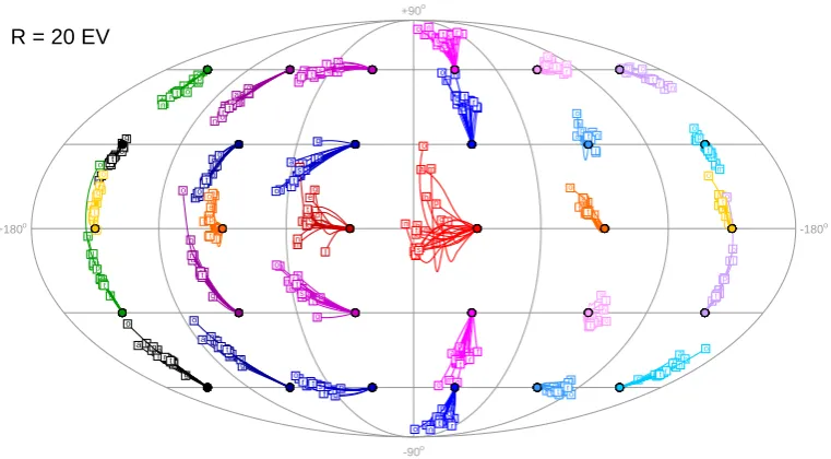
Figure 4.Backtracking of charged particles through the Galaxy starting from a regular grid of initial directions (dots). The resulting
directions outside of the Galaxy for particles with a rigidity of 20 EV are denoted by squares and the lines connecting the initial and final positions were constructed by performing backtracking at higher rigidities. Each of the letters (a)-(t) denotes a different GMF model that describes the synchrotron and RM data.
Figure 5.Minimum (left), average (middle) and maximum (right) magnification factor of the 20 GMF models studied in this work at
a rigidity of 10 EV.
impact of these models on the propagation of ultrahigh-energy cosmic rays in the Galaxy by backtracking charged particles from Earth to the edge of the Galaxy. The re-sults are shown in Fig.4for particle rigiditiesR≥20 EV (rigidity=energy/charge). As can be seen, the deflections predicted by different models are mostly confined within well-defined regions on the sky. If the variations studied in this work were bracketing the extreme possibilities for the large-scale configuration of the GMF, then one could use these results to construct a correction for the spatially varying average deflection based on all models and apply it to the arrival directions of UHECRs together with the uncertainty given by the spread of different model predic-tion. However, the variations studied here are most proba-bly not exhaustive and thus give only a lower limit on the current uncertainty of the inferred arrival direction of cos-mic rays at the edge of the the Galaxy. Nevertheless, in the era of high-statistics data from the Pierre Auger Ob-servatory and Telescope Array, the time seems ripe to use our current knowledge of the large-scale structure of the GMF to enhance studies of correlations between astro-physical sources and the arrival directions of cosmic rays (see also [33]).
In this context it is also worthwhile noting that not all extragalactic sources can be observed at Earth, because there exists no trajectory through the GMF that would
al-low a charged particle of certain rigidity to reach Earth from that direction [16,34,35]. This effect can be conve-niently described by themagnification factor[16,36] that quantifies the de- or increase of the flux received at Earth from a particular arrivial direction outside of the Galaxy due to the caustics of the GMF. Sky maps of the mag-nification factor can be constructed by performing many backtrackings from Earth on a fine isotropic angular grid and counting the number of trajectories leading from each extragalactic arrival direction to Earth [16,34,35]. The obtained magnification map satisfies Liouville’s theorem, since an isotropic flux of extragalactic cosmic rays will al-ways lead to an isotropic flux at Earth by construction.
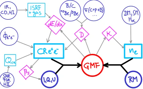
Figure 6. Sketch of the procedure to estimate the GMF from data (blue circles), models (azure squares) and auxiliary quanti-ties (magenta diamonds). See text for further explanation.
4 Summary
In these proceedings we have reported on progress in mod-eling the large-scale structure of the coherent and random magnetic field of the Galaxy. In addition to introducing new parametric models for the large-scale structure of the coherent GMF, we have studied the uncertainties of the underlying model assumptions inherent in the analysis as sketched in Fig.6.
In the first level of inference, the GMF is estimated from Q,U&I and RM data (thick blue circles), using mod-els of the thermal and cosmic-ray electron density (thick azure boxes). These models depend on further data (blue circles: DM, SM and Hα for ne and electron+positron
fluxes at Earth,Φe+e−, forncre). The interpretation of RM relies on an assumption about the correlation of ne and
B, which introduces a feedback loop into the inference process (magenta κ diamond). Another feedback loop is added by energy loss of cosmic-ray electrons in the Galaxy, dE/dx, which is in part due to synchrotron cool-ing in the GMF. Further model-dependencies of the energy loss are introduced by interstellar radiation fields (inverse Compton) and gas (ionization). In addition, a model of the spacial distribution of cosmic-ray sources,QCR, (based on sparse data on SNRs and their tracers), is needed to cal-culate three-dimensional density of cosmic-ray electrons. Even the data itself is not free of model assumptions, as some of the the estimates of the synchrotron emission Q,U&I use the spectral index of synchrotron radiationβS,
which in turn depends on the energy spectrum of cosmic-ray electrons. The diffusion coefficientDand its energy dependence is a direct effect of the GMF and in principle the diffusion coefficient could be self-consistently derived for any model of the GMF. However, usually Dis esti-mated from data on the secondary to primary ratios of the fluxes of cosmic-ray nuclei (e.g. B/C and10Be/9Be given fragmentation cross sectionsσin collisions of cosmic-ray nuclei with protons and helium of the ISM).
The 20 model variations presented here constitute a to-our-knowledge unique attempt to quantify the uncertain-ties of large-scale models of the GMF. Although our study does not necessarily cover the full range of models com-patible with the data, our preliminary conclusion is that
the derived GMF models vary significantly, but that for a typical application such as the backtracking of ultrahigh-energy cosmic rays, the data constrains the models enough to encourage further studies of the possibility of deriving GMF models with a realistic uncertainty.
Acknowledgments
We would like to thank Tess Jaffe for providing the simula-tions for the cosmic-ray electrons models from [27]. MU acknowledges the financial support from the EU-funded Marie Curie Outgoing Fellowship, Grant PIOF-GA-2013-624803 and the hospitality of CCPP/NYU, where part of this research was conducted. The research of GRF is sup-ported in part by the U.S. National Science Foundation (NSF), Grant NSF-1517319.
References
[1] A. C. Cummingset al.ApJ831(2016) 18.
[2] A. Shukurov, “Introduction to galactic dynamos,” in
Mathematical Aspects of Natural Dynamos, pp. 319–366.
2004.astro-ph/0411739.
[3] A. Neronov, “Galactic and intergalactic magnetic fields.”. these proceedings.
[4] R. Jansson and G. R. FarrarApJ757(2012) 14. [5] R. Jansson and G. R. FarrarApJ761(2012) L11. [6] M. Unger and G. R. FarrarPoS(ICRC2017)(2018) 558.
arXiv:1707.02339.
[7] J. C. Brownet al.ApJ663(2007) 258. [8] M. J. Reidet al.ApJ783(2014) 130. [9] C. L. Van Ecket al.ApJ799(2015) 35.
[10] J. Han, “The most updated results of the magnetic field structure of the milky way.”. these proceedings. [11] J. L. Han, R. N. Manchester, W. van Straten, and
P. DemorestApJS234(2018) 11.
[12] P. M. W. Kalberlaet al.ApJ794(2014) 90.
[13] P. M. W. Kalberla and J. KerpARA&A47(2009) 27. [14] E. S. Levine, L. Blitz, and C. HeilesApJ643(2006) 881. [15] B. Goldet al., [WMAP Collab.]ApJS192(2011) 15. [16] G. R. FarrarComptes Rendus Physique15(2014) 339. [17] E. N. Parker,Cosmical magnetic fields: Their origin and
their activity. Oxford University Press, 1979.
[18] K. Ferrière and P. TerralA&A561(2014) A100. [19] J. Jałochaet al.A&A566(2014) A87.
[20] E. S. Levine, C. Heiles, and L. BlitzApJ679(2008) 1288. [21] H. Men and J. L. HanActa Astron. Sinica44(2003) 151. [22] J. M. Cordes and T. J. W. Lazioastro-ph/0207156. [23] B. M. Gaensleret al.PASA25(2008) 184–200.
[24] J. Yao, R. N. Manchester, and N. WangApJ835(2017) 29. [25] M. J. Miller and J. N. BregmanApJ800(2015) 14. [26] R. Becket al.A&A411(2003) 99.
[27] R. Adamet al., [Planck Collab.]A&A596(2016) A103. [28] A. W. Stronget al.ApJ722(2010) L58–L63.
[29] E. Orlando and A. StrongMNRAS436(2013) 2127. [30] C. L. Bennettet al., [WMAP Collab.]ApJS208(2013) 20. [31] R. Adamet al., [Planck Collab.]A&A594(2016) A10. [32] C. G. T. Haslamet al.A&AS47(1982) 1.