Study of Stability Analysis of a Grid-Connected Doubly Fed Induction Generator (DFIG)-based small Wind Farm

Western University Western University

Scholarship@Western

Scholarship@Western

Electronic Thesis and Dissertation Repository

7-31-2013 12:00 AM

Study of Stability Analysis of a Grid-Connected Doubly Fed

Study of Stability Analysis of a Grid-Connected Doubly Fed

Induction Generator (DFIG)-based small Wind Farm

Induction Generator (DFIG)-based small Wind Farm

The University of Western Ontario Supervisor

Dr. Tarlochan S Sidhu

The University of Western Ontario Joint Supervisor Dr.Amirnaser Yazdani

The University of Western Ontario

Graduate Program in Electrical and Computer Engineering

A thesis submitted in partial fulfillment of the requirements for the degree in Master of Engineering Science

© Baishakhi Dhar 2013

Follow this and additional works at: https://ir.lib.uwo.ca/etd

Part of the Controls and Control Theory Commons, and the Power and Energy Commons

Recommended Citation Recommended Citation

Dhar, Baishakhi, "Study of Stability Analysis of a Grid-Connected Doubly Fed Induction Generator (DFIG)-based small Wind Farm" (2013). Electronic Thesis and Dissertation Repository. 1398.

https://ir.lib.uwo.ca/etd/1398

This Dissertation/Thesis is brought to you for free and open access by Scholarship@Western. It has been accepted for inclusion in Electronic Thesis and Dissertation Repository by an authorized administrator of

i

Study of Stability Analysis of a Grid-Connected Doubly Fed Induction Generator (DFIG)-based small Wind Farm

(Thesis format: Monograph)

by

Baishakhi Dhar

Graduate Program

In

Engineering Science

Department of Electrical and Computer Engineering

A thesis is submitted in partial fulfillment

of the requirements for the degree of

Master of Engineering Science

The School of Graduate and Postdoctoral Studies

University Of Western Ontario

London, Ontario, Canada

ii

Abstract

Wind is the most reliable, clean and fast-developing renewable energy source. The

DFIG-based variable speed wind turbine system is now the most popular in wind power

industry. With power being so in-demanding, a large wind farm needs to be developed to

produce more power from a stable system. But before such a large wind farm is installed,

better understanding is needed of the system’s intrinsic dynamic behavior, range of

stability region and parametric effects on system stability. Hence, a small wind farm with

two identical DFIG-based wind turbines connected to a grid network has been considered

for this study.

A detailed non-linear mathematical model of grid-connected single DFIG-based wind

turbine system as well as a grid-connected multi DFIG-based wind turbine system in a

dq-frame has been developed. Linearization of these non-linear mathematical models for

both the systems has been performed from the set of developed non-linear equations.

These two linearized dynamic models provide an analytical platform for determining the

robustness and stability of the two systems. The linearized models are then verified with

the simulation results of non-linear systems designed in a PSCAD/EMTDC environment.

This step is needed to check the performance accuracy of the linearized models. The

small-signal stability, the system’s parametric effects on stability and the modal analysis

of two developed linearized models have been studied. Participation factor analysis has

been employed to determine system parametric effects on each eigenmode. The intrinsic

dynamic behavior of a single wind turbine connected to a grid and multi wind turbines

connected to a grid (a small wind farm) are observed to be identical in nature at the same

iii

Acknowledgements

The author remembers with gratitude the constant guidance, suggestions and

encouragement forwarded by several respected persons and knows well that is not

possible to express indebtedness for all those valuable assistances by writing some lines.

She therefore, acknowledges in this page, the assistance rendered by all the concerned

persons, as a token her of gratitude.

The author likes to express her sincere gratitude and thanks to her supervisors Dr.

Tarlochan Singh Sidhu and Dr. Amirnaser Yazdani for their financial support, invaluable

supervision, kind and persistent valuable suggestion, advice, guidance, help and

encouragement from without which this thesis would not have been a reality.

The author is also thankful for financial support from Faculty of Engineering of the

Western University.

Finally, the author wishes to express her profound gratitude to her beloved husband for

providing the necessary atmosphere of understanding and support during most crucial

and disheartening moments.

iv

Table of Contents

Abstract ii

Acknowledgements iii

Table of Contents iv

List of Tables vii

List of Figures viii

Nomenclature xiii

Abbreviations xvi

Chapter 1: Introduction

1

1.1 Historical Background of Wind Power 1

1.2 Growth of Electricity Demand 2

1.3 Electricity Generation from Wind Power System 7

1.3.1 Inside of a Wind Turbine 7

1.3.2 Physics of Generating Electricity from Wind Energy 11

1.3.3 Different Types of Wind Turbine 15

1.4 Survey of Existing Work 20

1.5 Scope of the Thesis 22

1.6 Thesis Objectives 22

1.7 Methodology 23

v

Chapter 2: Mathematical Modeling and Control of Grid-Connected

DFIG- based Wind Energy Conversion System

2.1 Grid-Connected Single DFIG-based Wind Power System 26

2.1.1 Stator Flux Observer 28

2.1.2 Torque/ Flux Controller 30

2.1.3 Phased Locked Loop (PLL) 33

2.1.4 Back-to-back Converter & DC Bus Voltage Controller 34

2.1.5 Distribution Network 38

2.2 Grid-Connected Two Identical DFIG-based Wind Power Systems 39

2.3 Model Linearization 41

2.4 Summary and Conclusions 45

Chapter 3: Model Validation and Simulation Result

47

3.1 Case Study 1 48

3.2 Case Study 2 57

3.3 Summary and Conclusion 66

Chapter 4: Modal Analysis- System Parametric Effects

67

4.1 Brief Description of Stability & Modal Analysis 67

4.2 Sensitivity Analysis At Very Low Linking Inductances 69

vi

4.2.2 Eigenvalue, Frequency of Oscillation and Damping Factor 74

4.3 Sensitivity Analysis at Very High Linking Inductances 82

4.4 Summary and Conclusion 84

Chapter 5: Summary, Conclusions and Future Works

86

5.1 Summary and Conclusions 86

5.2 Future Work 88

References 89

Appendices

93

Appendix A 93

Appendix B 95

vii

List of Tables

Chapter 1

Table 1.1: Three different scenarios for global cumulative wind power capacity

(2011-2030)

Chapter 4

Table-4.1: Participation factor analysis at wind speed = 13.5 / and linking

inductance = 1 μ

Table-4.2: Participation factor analysis at = 13.5 / and = 13.5 /

and linking inductance = 1 μ, = 1 μ

Table-4.3: Participation factor analysis at = 13.5 / and = 7 / and

linking inductance = 1 μ, = 0.5 μ

Table-4.4: Change in eigenvalues λ29 of linearized model of Figure 2.1 and λ53 and

viii

List of Figures

Chapter 1

Figure 1.1 Global cumulative installed wind capacity (1996-2012)

Figure 1.2 Global cumulative wind power capacity (2011-2030)

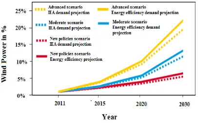
Figure 1.3 Wind power share of global electricity demand (2011-2030)

Figure 1.4 Schematic diagram of wind turbine subsystems

Figure 1.5 Power coefficient Cp vs. tip speed ratio graph

Figure 1.6 Graph of turbine power in per unit vs. turbine speed in per unit.

Figure 1.7 (a) Schematic diagram of horizontal axis wind turbine. (b) Schematic

diagram of vertical axis wind turbine.

Figure 1.8 Schematic diagram of constant speed wind turbine system.

Figure 1.9 (a) Schematic diagram of DFIG variable speed wind turbine system. (b) Schematic diagram of FRC variable speed wind turbine system.

Chapter 2

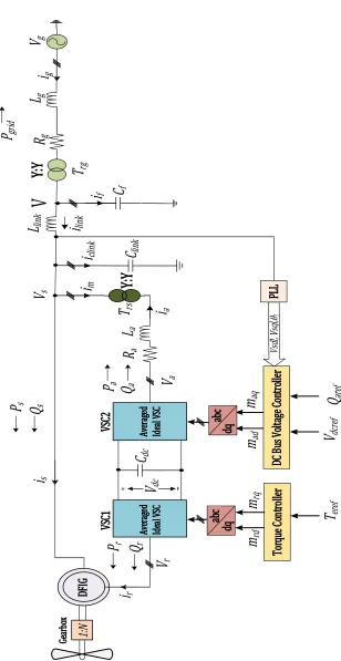
Figure 2.1 Schematic diagram of grid-connected DFIG-based single wind power

system

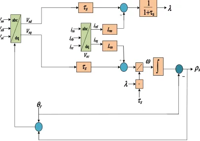
Figure 2.2: Schematic diagram of stator flux observer

Figure 2.3: Schematic diagram of rotor q-axis reference current generator

Figure 2.4: Block diagram of machine rotor current control loop

ix

Figure 2.6: Schematic diagram of current control loop for grid side VSC System

Figure 2.7: (a) Schematic diagram of DC voltage controller with feed-forward scheme

(b) Reference signal generator

Figure 2.8: Schematic diagram of grid connected two DFIG-based wind power

systems

Chapter 3

Figure 3.1: Responses of rotor speed of wind turbines (a) Response of wind turbine of

Figure 2.1 (b) Response of Wind Turbine 1 of Figure 2.8 (c) Response of

Wind Turbine 2 of Figure 2.8

Figure 3.2: Responses of dc link voltages of ac-dc-ac back to back VSCs (a) Response

of Figure 2.1 (b) Response of Wind Turbine 1 of Figure 2.8 (c) Response

of Wind Turbine 2 of Figure 2.8

Figure 3.3: Responses of stator fluxes of wind turbines (a) Response of wind turbine

of Figure 2.1 (b) Response of Wind Turbine 1 of Figure 2.8 (c) Response

of Wind Turbine 2 of Figure 2.8

Figure 3.4: Responses of electrical torques of wind turbines (a) Response of wind

turbine of Figure 2.1 (b) Response of Wind Turbine 1 of Figure 2.8 (c)

Response of Wind Turbine 2 of Figure 2.8

Figure 3.5: Responses of active power of rotor side converters (a) Response of Figure

2.1 (b) Response of Wind Turbine 1 of Figure 2.8 (c) Response of Wind

x

Figure 3.6: Responses of active power of grid side converters (a) Response of Figure

2.1 (b) Response of Wind Turbine 1 of Figure 2.8. (c) Response of Wind

Turbine 2 of Figure 2.8.

Figure 3.7: Responses of reactive power of rotor side converters (a) Response of

Figure 2.1 (b) Response of Wind Turbine 1 of Figure 2.8 (c) Response of

Wind Turbine 2 of Figure 2.8

Figure 3.8: Responses of reactive power of grid side converters (a) Response of

Figure 2.1 (b) Response of Wind Turbine 1 of Figure 2.8 (c) Response of

Wind Turbine 2 of Figure 2.8

Figure 3.9: Responses of rotor speed of wind turbines (a) Response of wind turbine of

Figure 2.1 (b) Response of Wind Turbine 1 of Figure 2.8 (c) Response of

Wind Turbine 2 of Figure 2.8

Figure 3.10: Responses of dc link voltages of ac-dc-ac back to back VSCs (a) Response

of Figure 2.1 (b) Response of Wind Turbine 1 of Figure 2.8. (c) Response

of Wind Turbine 2 of Figure 2.8.

Figure 3.11: Responses of stator fluxes of wind turbines (a) Response of wind turbine

of Figure 2.1 (b) Response of Wind Turbine 1 of Figure 2.8. (c) Response

of Wind Turbine 2 of Figure 2.8.

Figure 3.12: Responses of electrical torques of wind turbines (a) Response of wind

turbine of Figure 2.1 (b) Response of Wind Turbine 1 of Figure 2.8 (c)

xi

Figure 3.13: Responses of active power of rotor side converters (a) Response of Figure

2.1 (b) Response of Wind Turbine 1 of Figure 2.8 (c) Response of Wind

Turbine 2 of Figure 2.8

Figure 3.14: Responses of active power of grid side converters (a) Response of Figure

2.1 (b) Response of Wind Turbine 1 of Figure 2.8 (c) Response of Wind

Turbine 2 of Figure 2.8

Figure 3.15: Responses of reactive power of rotor side converters (a) Response of

Figure 2.1 (b) Response of Wind Turbine 1 of Figure 2.8 (c) Response of

Wind Turbine 2 of Figure 2.8

Figure 3.16: Responses of reactive power of grid side converters (a) Response of

Figure 2.1 (b) Response of Wind Turbine 1 of Figure 2.8 (c) Response of

Wind Turbine 2 of Figure 2.8

Chapter 4

Figure 4.1: Eigenvalue loci for change in linking inductances (a) λ1,2 and λ3,4 for single- turbine connected with grid (b) λ1,2 and λ3,4 for two-turbine system connected with grid. (c) λ5,6 and λ7,8 for two-turbine system connected to a grid

Figure 4.2: Frequency of oscillation (fosc) and damping Factor (ζ) of eigenvalues of Figure 4.1 (a) Frequency of oscillation (fosc) (b) Frequency of oscillation

xii

Figure 4.3: Graph for change in linking inductances with real part of dominant

eigenvalue (σ) of linearized model grid-connected single-turbine system and grid- connected two-turbine systems, with change in linking

inductances

Figure 4.4: Eigenvalue loci for change in wind speed (a) λ29 for single-turbine connected to a grid. (b)λ53 for two-turbine system connected to a grid (c)

λ54 for two-turbine system connected to a grid

Figure 4.5: Graph for change in wind speed with real part of dominant eigenvalue for

(a) Linearized model of Figure 2.1 and (b) Linearized model of Figure

2.8.

Figure 4.6: Graph for change in system parameters with real part of dominant

eigenvalue (a) Change in linking inductances (b) Change in wind speed

Figure 4.7: Dominant eigenvalue loci from 6 m/s to 14 m/s at linking inductance

0.00032 H (a) Linearized model of grid-connected single-turbine and (b)

xiii

Nomenclature

Stator voltage

Stator current

Rotor current

Rotor voltage

Grid-side converter ac-side terminal voltage

Grid-side converter ac-side terminal current

Rotor active power

Rotor reactive power

Stator active power

Stator reactive power

Ac-side terminal active power of grid-side converter

Ac-side terminal reactive power of grid-side converter

Magnetizing inductance

Stator inductance

Rotor inductance

Rotor resistance

Stator resistance

xiv

s1 Subscript used for DFIG-based wind turbine 1

s2 Subscript used for DFIG-based wind turbine 2

Subscript used for direct axis component of a variable

! Subscript used for quadrature axis component of a variable

Voltage at PCC

"# Grid steady state angular frequency

" Rotor angular speed

$ Moment of inertia

% Stator time constant

% Rotor time constant

&'( Turbine torque

&) Electrical torqur

Linking inductance between machine and PCC

*'+ Turn ratio of transformer &

*', Turn ratio of transformer &,

, Resistance at Transmission line

Grid-side converter ac-side terminal resistance

Grid-side converter ac-side terminal inductance

, Grid Voltage

xv

-/+ DC side capacitor of two VSC

/+ Voltage across -/+

- Shunt capacitor at machine and linking inductance meet point

+ Current across capacitor -

Current across

, Inductance at Transmission line

" Angular frequency of PLL reference frame

0 Reference frame angel of PLL

1 Stator flux phase-angle

" Angular frequency of stator flux

2 Damping factor

xvi

Abbreviations

DFIG Doubly Fed Induction Generator

VSC Voltage Source Converter

USSR Union of Soviet Socialist Republics

GWEO Global Wind Energy Outlook

HAWT Horizontal Axis Wind Turbine

VAWT Vertical Axis Wind Turbine

FRC Fully Rated Converter

IGBT Insulated Gate Bipolar Transistor

PWM Pulse Width Modulation

PCC Point of Common Coupling

1

Chapter 1

Introduction

In recent years, nations have sought alternative renewable energy resources to meet their

rapidly growing demands of power, mainly due to the rapid increase of fuel costs and

rising pollution levels. Continuously trimming down traditional energy resources as well

as preservation of non-renewable energy resources are the two main causes of increased

fuel costs. Pollution levels keep increasing, mainly due to long-term use of fossil fuels

and increase in population. Different types of renewable energy sources are Biomass

Energy, Hydro-Power Energy, Solar Energy, and Wind Energy. Among all these

renewable energy sources, wind energy is most in-demand, as wind is a clean source of

energy, with no waste products created during wind power generation. Wind power

generation does not need any fuel and is able to supply considerable level of energy to

meet world demand.

1.1

Historical Background of Wind Power

Wind power has been used from many years, since humans first started of use of sailboats

and sailing ships. Ackermann [1] stated that at least from the 7th century BC, vertical axis

windmills were used in the Afghan highlands to grind grain. It has been found that

horizontal axis windmills were used in about 1000 AD by Persian, Chinese and Tibetan

2

Central Europe from Persia and the Middle East. In around 1150 AD, this type of

windmill reached England; in 1180 AD it reached France, in 1222 AD Germany, and in

around 1259 AD, Denmark. Between the 12th to 19th centuries, windmill performance

was constantly enhanced, and by the end of the 19th century, typical European windmills

were developed, with a rotor of 25 m in diameter, and stocks reaching up to 30 m [1]. In

the mid-1700’s, Dutch settlers established windmills in America [2]. By 1800, 90% of

power used in industry in the Netherlands was from wind power [1]. In the United States

of America (USA), between 1880 and 1930, around 6.5 million units of windmills were

installed by different companies to provide water for farm animals [2].

1.2

Growth of Electricity Demand

Burton et al. [3] stated, 12 kW DC windmill generator was developed to produce

electricity in the late 19th century by Brush in USA and this research was carried out by

LaCour in Denmark. In 1931, Union of Soviet Socialist Republics (USSR) constructed

100 kW- 30 m diameter Balaclava wind turbine, which was the first utility scale wind

turbine in the world. In 1941, in USA, 1250 kW Smith-Putnam wind turbine was

developed that had a steel rotor with diameter of 53m, full-span pitch control and

flapping blades to reduce loads. This wind turbine was operated for 1100 hours before a

blade spar failed in 1945. This wind turbine remained the largest wind turbine for around

40 years.

A hollow blade, open at tip with 24 m diameter pneumatic wind turbine was constructed

in early 1950s in UK to draw air through the tower. In 1956 and in 1963, 200 kW with 24

3

constructed in Denmark and in France, respectively. In between 1950s and 1960s a

number of modern, lightweight turbines were developed by U. Hutter in Germany. In

spite of this technological progress, it was seen that for much of the 20th century, world

had little interest to use wind energy other than in remote residences for battery charging

[3].

After a sudden price hike of oil occurred in 1973 because of inadequate fossil-fuel

resources, countries like USA, UK, Germany, Sweden took serious steps with a large

number of Government-funded programs of research, development and manifestation to

investigate cost effective sources of energy. As a result of fact, in between 1975 and

1987, a series of prototype wind turbines starting with 38 m diameter 100 kW Mod-0 and

97.5 m diameter 2.5 MW Mod-5B, respectively, were constructed in USA [3]. Nearly at

the same time a 4 MW vertical-axis Darrieus wind turbine and a 34 m diameter Sandia

vertical-axis wind turbine were constructed, in Canada and in USA, respectively. Another

vertical-axis wind turbine with straight blades using ‘H’ type rotor was designed by Peter

Musgrove and this model was constructed in UK that had a capacity to generate 500 kW

power. An entire structure of 3 MW horizontal axis wind turbine was designed and tested

in USA, in 1981 that used hydraulic transmission, an alternative to yaw drive [3]. In

mid-1980s, a large number of small wind turbines with capacity less than 100 kW were

installed in a wind farm with a maximum total capacity of 1.5 MW in California [4]. But

for some time, the selection of the number of blades remained undecided and the turbines

were constructed with a maximum of three blades. Installed wind turbine capacity was

increased from 2.5 GW in 1995 to 12 GW by 2001 [3]. Figure 1.1 shows a statistical

4

growth of wind energy has been noticed [5]. From 1996 to 2012, an exponential increase

of the growth of global cumulative installed wind capacity is observed in Figure 1.1.

Figure 1.1: Global cumulative installed wind capacity (1996-2012) [5]

As per the 2012 report on global wind energy outlook (GWEO), the growth of global

cumulative wind power capacity with three different scenarios in MW unit and wind

power share of global electricity demand in percentage, have been plotted for the time

period 2011 to 2030, in Figure 1.2 and in Figure 1.3, respectively; while Table 1.1 also

lays out the power generation for the three different scenarios [6]. On the basis of current

directions and intentions from both national and international energy and climate policy,

the “New Policies” scenario is analyzed. The factors related to “Moderate Policies”

scenario are mostly similar to “New Policies” scenario; but it also comprises of all policy

5

the commitments of the emission reductions [6]. The most aspiring scenario is

‘Advanced Policies’ scenario. This consists of unambiguous commitment to renewable

energy in line with industry recommendations, the political will to commit to appropriate

policies and the stamina to stick with them [6].

Figure 1.2: Global cumulative wind power capacity (2011-2030) [6]

IEA demand projection of new policies scenario was obtained from Figure 1.3. The

projection showed that the wind power share of global electricity demand will increase

from 3.5% to 4.7% by 2015 and is projected to be 8% by 2030. But, considering the

energy efficiency demand projection of the same scenario, the demand will reach 9% by

6

Table 1.1: Three different scenarios for global cumulative wind power capacity

(2011-2030) [6]

Different Scenarios 2011 2015 2020 2030

New Policies Scenario

[MW]

237,699 397,859 586,729 917,798

Moderate Scenario [MW] 237,699 425,155 759,349 1,617,444

Advanced Scenario [MW] 237,699 530,945 1,149,919 2,541,135

7

1.3

Electricity Generation from Wind Power System

Wind turbine generates electricity from wind power to drive electrical machine. If a

machine converts kinetic energy of the wind to mechanical energy, and then, this

mechanical energy is used to generate electrical energy, that machine is defined as the

wind power plant or wind turbine. A detailed description of some fundamental facts of

wind turbine such as basic parts, principle of operation and etc. are discussed to get an

idea of modern wind turbine system.

1.3.1 Inside of a Wind Turbine

Wind turbine mechanism is exactly the reverse of a fan. Fans use electricity to generate

wind, whereas wind turbines use wind to generate electric power. The rotor of wind

power system is connected to the main shaft, which spins a generator to produce

electricity [7]. Figure 1.4, illustrates a detailed view of the inside of a wind turbine

system and its components. Major components of a typical wind turbine system are as

follows:

Rotor: The most important part, from both performance and overall cost stand point, of a

wind turbine is its rotor; that consists the hub, the high tech blades and a spinner [9,10].

Heaviest components of wind turbine are the hub as it is made of ductile cast iron. For a 2

MW modern wind turbine the weight of the hub is normally in between 8 to 10 tons. The

hub can absorb a high level of vibration. The nose cone helps to cover the hub and also to

protect it slightly the hub from the environment. Nose cone is made from balsa wood,

8

Figure 1.4: Schematic diagram of wind turbine subsystems [8]

One of the most critical and premeditated component of wind turbine system is its blades.

The composition of the blades is same as that of the nose cone. To enhance performance

of wind turbine in various wind conditions different types of blade are created for a

single-turbine. 61.5 m long blade is the world’s longest blade made for a 5 MW turbine

9

Drive Train: This part consists of a low speed shaft, a high speed shaft, a gear box, one

or more couplings, support bearings, a brake and a rotating part of generator. The low

speed shaft is made on rotor side while the high speed shaft is on the generator side [9].

This drive train is electricity generating system of a wind power system. Gearbox steps

up the rate of rotation of the rotor from a low value to a high value suitable for electric

generator. As a gear box handles the frequent changes in torque due to changes in wind

speed, it must be robust. A lubrication system is used to minimize the wear needed for the

gear box system. Mainly parallel shaft and planetary, these two types of gear box are

used in wind turbine system. Planetary type gear box is used normally in large wind

turbine over 500 kW. Mainly induction generator based wind turbines need gearbox. To

stay away from mechanical problem related to gear box, some wind turbines use a direct

drive system which connects the rotor directly to a permanent magnet generator [9,10].

Nacelle: A box-like component at the top of tower is connected to the rotor, is called the

nacelle. This contains around 8000 components of wind power system like generator,

main frame, etc. Nacelle saves the internal components of turbine from weather and is

made of fiberglass. The nacelle cover is fixed firmly to the main frame, which also

supports all the other components inside the nacelle. The main frames provide proper

alignment of drive train components and are also able to withstand large fatigue loads

10

Yaw System: To keep the rotor shaft properly aligned with the wind a yaw system is

needed. A large bearing that connects the main frame to the tower is the main component

of yaw drive system. The yaw drive system uses either an electric or hydraulic motor

which drives a pinion gear on a vertical shaft through a reducing gearbox. Typically a

yaw drive system is used with an upwind wind turbine system, whereas downwind wind

power systems are often free from yaw systems. [9]. A brake is also used in a yaw drive

system to stop a turbine from turning and stabilizing it during normal operation [10].

Generator: To get constant rotational speed, mainly induction or synchronous generators

are used with all wind turbines. Power electronic converters are used with the generators

to run wind turbines at variable speed. Squirrel cage induction generators (SQIG) can be

used with many grid-connected wind turbines, due to it being rugged by nature, low cost,

and driven in a narrow range of speeds, slightly higher than its synchronous speed.

Nowadays, doubly fed induction generators (DFIG) have gained popularity in variable

speed applications. Main advantages of DFIG are simple configuration, over a wide range

of wind speed; wind turbines work efficiently [9].

Tower and Foundation: For use of maximum wind nacelle and generator are situated on

the top of the tower [10]. In recent times, lattice towers, concrete towers and free standing

steel tube towers are most popular. Depending on the site character, tower is selected.

Normally height of a tower varies from 1 to 1.5 times of the rotor diameter. Stiffness of

tower plays an important role in wind turbine system dynamics as vibration occurs

11

considered to have significant effect on power fluctuations, turbine dynamics and noise

generation [9].

Controls: To get proper functioning from wind turbine, few instruments like sensors,

controllers, power amplifiers, actuators and some intelligent devices like microprocessors

and computers are used as control system. Sensors are used to sense and give feedback of

wind speed, direction, flow, current, voltage, rotor speed, temperature, vibration levels

etc. Electrical circuits and mechanical systems act as controllers to control all the

parameters. Different types of switches, hydraulic pumps, electrical amplifiers etc. are the

parts of power amplifiers. Motors, magnets, solenoids etc. act as actuators. Few

intelligent devices like computers and microprocessors are used to process the inputs of

turbine to get proper function from turbine and also at an emergency situation, which

help to override the controller to safe overall system [9, 10].

The most fundamental and major components of a typical wind turbine connected to a

grid is discussed above. Other than these components, some other components like

transformers, power electronic converters and pitch motors etc. are used depending on the

complexity of the system to get proper functionality.

1.3.2 Physics of Generating Electricity from Wind Energy

Wind energy is one form of solar energy generated because of temperature and as well as

pressure differences in the atmosphere, the rotary motion of the earth, and the

irregularities of the earth's surface. Sun heats up the air, forcing the air to rise; this causes

12

to balance the differences. Wind turbine first catches wind’s kinetic energy which helps

to drive generator to produce electricity [11]. The kinetic energy in air with mass

moving with velocity is given by [12]:

34 =

_(1.1)

The power in wind is the Kinetic energy per unit time and as is expressed as:

=

5

,

(1.2)

where

5 =

/'

=

The mass flow rate /

/' is:

/

/'

= 1>

,

(1.3)

where 1 and > are defined as air density and the rotor effective area, respectively.

Finally, the wind power equation is:

=

1>

(1.4)

Power extracted from wind by the turbine blades is the difference between upstream and

downstream wind powers and is given by:

=

(

−

)

(1.5)

where is the actual wind speed or upstream wind velocity at the entrance of the rotor

blades and _B is the downstream wind velocity at the exit of rotor. The mass flow rate of

the air through rotating blades is then expressed as:

6 789: ;6<=

= 1>

2

(1.6)

13

=

F1>

K (

−

)

(1.7)

Equation (1.7) is modified to be:

=

1>

LI_MHMJNOPL_MHMJNQR

,

(1.8)

where

-

=

MJ

MHNOPLMHMJN Q

R

(1.9)

is the power coefficient of the rotor. -_S, is the fraction of upstream wind power.

Finally the turbine power _'( from equation (1.8) is rewritten to be:

=

1>

-

(1.10)

The power coefficient, -_S, is thus a dimensionless parameter and is the ratio of turbine

power _'( to that of wind power .

-

=

(1.11)

The maximum value of -_S is defined by Betz limit and is 0.59, as Betz limit states that a

turbine can never extract more than 59.3% of wind power. Practically -_S varies from

25% to 40% [13] for the wind turbine. -_S, is a function of the blade pitch angle, W_X'+Y

and the tip speed ratio, _Z/). _Z/), is defined as the ratio of upstream wind speed

and downstream wind speed _B.

=

GJ

(1.12)

This, _Z/) can also be expressed in terms of turbine angular speed, "_'(, turbine radius,

;, and wind speed, , and is given as :

14

The relationship between -_S and tip speed ratio _Z/) is then established by using the

blade theory of turbine and is given by [14]:

-

=

(

− 0.022W

− 5.6)=

(1.14)

Figure 1.5 shows the changing behavior of the power coefficient -_X with the changing tip speed ratio _Z/). It can be stated from this figure that, maximum -_X is only achieved at a single tip-speed ratio and for a fixed rotational speed of the wind turbine; this happens only at one single wind speed.

Figure 1.6 shows the nature of the graph for turbine power in per unit value with the

change in turbine speed which is in per unit value at different wind speed. This wind

speed varies from 6 m/s. to 14 m/s. The maximum turbine power in Figure 1.6 is seen to

change for different wind speed.

15

Figure 1.6: Graph of turbine power in per unit vs. turbine speed in per unit

1.3.3 Different Types of Wind Turbine

Wind turbines are classified in two ways. Firstly, the classification depends on the

position of the rotor axis of wind power system and secondly, it depends on the variation

of wind speed. Wind turbine can be classified into horizontal axis wind turbine (HAWT)

and vertical axis wind turbine (VAWT) [15]. Depending on the variation of wind speed

wind turbines are also classified into constant speed wind turbine and variable speed

wind turbine [16].

HAWT: Most popular commercial wind turbine connected to a grid, in recent times is

16

turbine, the rotor shaft and electrical generator are placed at the top of the tower where

wind is less turbulent and wind has more power. Figure 1.7 (a) shows the schematic

diagram of HAWT [15].

Figure 1.7: (a) Schematic diagram of horizontal axis wind turbine. (b) Schematic

diagram of vertical axis wind turbine [15]

VAWT: The main rotor shaft in VAWT is placed vertically in the wind turbine system.

Figure 1.7 (b) shows Darrieus rotor type vertical axis wind turbine system which is the

most popular type VAWT [15]. The main advantages of this kind of wind turbines are

that, the generators and gearboxes are easy to repair and perform maintenance operation

of the components as they are placed close to ground, and also this turbine can catch the

wind from all direction without any yaw system. Though there are advantages, but this

type of wind turbine has many disadvantages like, low starting torque, sensible to design

17

applications such as battery charging, as output power is very low; thus, minimizes the

popularity of VAWT comparing with HAWT [17].

Constant Speed Wind Turbine: This type of turbine is simple in design and is

composed of a gearbox, a low speed shaft, a high speed shaft and an asynchronous

generator. Figure 1.8 presents the schematic diagram of a constant speed wind turbine

system. Mainly squirrel-cage induction generator is used to generate power from such

type of system [13]. For this turbine system, a power-electronic converter is not needed

since the system works at constant speed, and therefore it is structurally simple.

Synchronous frequency is imposed by the grid to the machine because the generator is

directly interfaced with the utility grid through a turbine transformer machine. The

rotational speed of the asynchronous generator is not exactly constant and varies within

±3% to ±8% of the synchronous speed which is very small, so this type of turbine is

18

Gearbox

Machine

Figure 1.8: Schematic diagram of constant speed wind turbine system [16]

Variable Speed Wind Turbine: Though structurally complex, this type of wind turbine

system is more popular comparing with constant speed wind turbine as maximum energy

can be generated due to the variability in speed of the turbine system. A solid-state power

converter is always used to interface the machine to the transmission system. There are

two different types of variable speed wind turbines that are most common nowadays.

These are: wind turbine with doubly fed induction generator (DFIG) and wind turbine

with fully rated converter (FRC) based on a synchronous or induction generator [13].

• DFIG Wind Turbine: Power can be delivered to the grid through both stator and

rotor of the machine for this type of variable speed wind turbine system. Depending

on the rotational speed of the generator the rotor can also absorb power [13]. The

rotor absorbs power from the grid through power converter when the operating speed

of generator is lower than the synchronous speed and it delivers power to the grid

when the generator operates above the synchronous speed [13]. A schematic diagram

of this type of turbine is shown in Figure 1.9 (a). A controllable voltage is injected

19

AC/DC IGBT based voltage source converters (VSCs), linked by a DC bus is

interfaced in between the rotor winding and electrical network to decouple

transmission line electrical frequency from rotor mechanical frequency. Thus, the

variable speed operation of wind turbine is possible [13].

• FRC Wind Turbine: Figure 1.9 (b) shows a schematic diagram of FRC wind turbine

system. A wide range of electrical generators like wound rotor synchronous

generator, permanent magnet generator, induction generator etc. can be used for this

type of turbine system. Use of the gearbox is optional for FRC wind turbine system.

Variable speed operation can be performed as the dynamic operation of electrical

generator is effectively separated from the electrical network through power

converters [13]. A diode rectifier or a PWM VSC can be used as generator side

converter and only PWM VSC can be used as grid side converter. Each type of

converter can independently deliver or absorb reactive power independently. Mainly

DC bud voltage is controlled by the grid side converter whereas generator side

converter controls the torque applied to the generator. But reverse control strategy is

20

Gearbox

Machine

AC/DC/AC Power Electronic Converter

(a)

Gearbox

Machine AC/DC/AC Power

Electronic Converter

(b)

Figure 1.9: (a) Schematic diagram of DFIG variable speed wind turbine system [16] (b) Schematic diagram of FRC variable speed wind turbine system [16]

1.4

Survey of Existing Work

As shown in section 1.2, the demand for wind power to meet global electricity demand

has been increasing. In Recent years, variable-speed DFIG-type wind-power systems

have become commercially very popular for generating wind power, but because of the

erratic nature of wind velocity, extensive research has been done to analyze system

stability and sensitivity for the changes of different system parameters to get efficient and

economic production of wind energy from a stable wind-power-generating system. A

brief review of previous research shows the relation between system modeling and

stability analysis of a DFIG wind turbine system. Different models of grid-connected

21

formulated mathematically and compared with each other using eigenvalues and

participation factor analysis [18]. Rouco and Zamora [19] developed detailed non-linear

and corresponding linear mathematical models of DFIG systems for wind power

applications. They offered a reduced order model of the detailed models using

eigenvalues of the state matrix and corresponding participation factor analysis. A

comparative study has also been carried out on the detailed models and the proposed

reduced order models [19]. Modal analysis, with a 7th order grid-connected DFIG-based

system, has been performed for, better understanding of basic dynamics of the system,

model justification and control system design [20]. This study was carried out by

changing the modal properties for different operating points, grid strengths and system

parameters. [21] has designed damping controllers of DFIG for damping

electromechanical oscillation by eigenvalue sensitivity analysis with respect to some

parameters. A detailed mathematical model of DFIG has been developed, to analyze

eigenvalue sensitivity with respect to machine and control parameters, and to evaluate

their impacts on system stability; it has also been shown that without proper controller

tuning, a Hopf bifurcation can occur for various reasons [22].[23] has presented a study

on participation factor analysis using eigenvalue of a mathematically developed

DFIG-based wind-power unit interfaced with the grid through a series compensated

transmission lines. The influence of the system parameters on stability of the system has

22

1.5

Scope of the Thesis

As the literature review makes clear, considerable research has been carried out to

analyze system stability and modal analysis in a single DFIG-based-turbine connected to

a grid. However, a very few research has been performed to clarify the intrinsic dynamic

behavior of a wind farm comprised of multi-turbine systems. As wind power is very

much in demand nowadays, being a non-conventional energy resource to generate

electric power, it is necessary to construct large wind farms that can produce maximum

power from a stable system. Hence, this thesis is motivated by the desire to contribute to

the better understanding of the intrinsic dynamic behavior, range of stability region and

system’s parametric effects on the system stability of a small wind farm. To achieve

these, a small wind farm with two identical DFIG-based wind turbines connected to a

grid network needs to be established.

1.6

Thesis Objectives

The objectives of the thesis are

• To develop a linearized mathematical model from a non-linear DFIG-based single

wind power system connected to a grid. Also on the basis of this model, to

establish a linearized model of a small DFIG-based wind farm connected to a

distribution network.

• To validate the established linearized mathematical models by comparing the

simulation results from both the linear and non-linear models.

• To study and analyze the system stability, eigenvalue sensitivity and modal

23

1.7

Methodology

The following methodology is used in order to carry out the objectives:

• non-linear analytical models of a grid-connected DFIG-based single-turbine and

a grid-connected DFIG-based multi-turbine systems are established.

• to clarify the dynamic behavior of both the systems, linearized mathematical

models are developed from the non-linear models.

• to validate the linearized models for a single-turbine system and the wind farm,

the simulation results of the linear and non-linear models are compared

separately.

• to examine the system stability and fundamental dynamic behavior, participation

factor analysis and eigenvalue sensitivity analysis are performed for different

operating conditions and system parameters.

1.8

Thesis Layout

Thesis is organized in the following manner:

• Chapter 2 develops mathematical linearized models of a DFIG-based wind turbine

system connected to a grid and a small wind farm involving two identical DFIG-

based wind turbines connected to a grid around an equilibrium point, including all the

control system blocks, system and network equations, based on non-linear models.

• Chapter 3 deals with the validation of linearized system performance with non-linear

models developed in a PSCAD/EMTDC environment for a single-turbine connected

24

• Chapter 4 presents system stability analysis and modal analysis of the linearized

models developed in Chapter 2 to determine the intrinsic dynamics for model

justification and for useful control system block design in order to achieve wide range

system stability with maximum output power.

• Finally, Chapter 5, summarizes and concludes the thesis and presents the scope of

25

Chapter 2

Mathematical Modeling and Control of

Grid-Connected DFIG-based Wind Energy Conversion

System

This chapter develops a non-linear mathematical model of a DFIG-based wind power

system connected to a grid. A linearization is performed on the same system for small-

signal stability analysis. Two of these, identical DFIG-based wind power systems are

then considered to be connected in parallel with a distribution network through a Point of

Common Coupling (PCC). The resulting design is then referred to as a small wind farm

connected to a grid. A non-linear mathematical model of this wind farm is then

developed and linearization is performed.

The non-linear equations for both the models established on “dqo” frame are used, which

simplify the analysis of three phase circuits, transform AC quantities into DC quantities,

decouple DFIG torque and flux, and also avoid the time varying mutually coupled

inductances of the overall systems [16]. From each of the system equations, the o-axis

components are eliminated. The variables with the d- and q-axis components are denoted

26

Each of the individual wind power systems consists of individual control system blocks,

back-to-back voltage source converters (VSCs), and a phase locked loop (PLL). An

in-depth description of each of these blocks for both in linear and non-linear mathematical

forms is presented here.

2.1

Grid-Connected Single DFIG-based Wind Power System

Figure 2.1 presents a schematic diagram of a grid-connected single DFIG-based wind

turbine system. All the parametric values used for the system are mentioned in the

appendix A. The turbine is interfaced with the grid through a linking inductance, , a

transformer, &_,, and a transmission line where an ideal voltage source, _, , is the grid as

mentioned in Figure 2.1. The high voltage side of the &_, is connected with _,. The

stator of the DFIG is directly connected to , while the rotor is connected through the

ac-dc-ac back-to-back VSCs to . Figure 2.1 shows the two back-to-back converters,

rotor side and grid side converters that are referred to as VSC1 and VSC2, respectively.

Thus capacitors, - and -_. provide a low-impedance path for switching harmonics,

which are generated by VSCs. The voltage at PCC is , where and &_,, are

connected. The transmission line consists of resistance, _,, and inductance, _,,

connected in series. The mechanical dynamics of Figure 2.1 is described by

$

/'

= &

− &

,

(2.1)

where $ is the moment of inertia, " is the machine rotor speed, &_'( is considered to be

27 To rqu e C on tro ller To rqu e C on tro ller To rqu e C on tro ller To rqu e C on tro ller Ge arb ox Ge arb ox Ge arb ox Ge arb ox Av era ged Av era ged Av era ged Av era ged Ide al V SC Ide al V SC Ide al V SC Ide al V SC Av era ged Av era ged Av era ged Av era ged Ide al V SC Ide al V SC Ide al V SC Ide al V SC DC Bu s V olt age Co ntr olle r DC Bu s V olt age Co ntr olle r DC Bu s V olt age Co ntr olle r DC Bu s V olt age Co ntr olle r VS C VS C VSCVSC 1111 VS C VS C VSCVSC 2222 DF IG DF IG DF IG DF IG PL L PL L PLLPLL dqdqdqdq abcabcabcabc

V

C

V

P

_Q

P

P

a

Q

i

i

Q

V

R

i

L

m

V

m

m

m

T

C

i

i

i

L

C

i

T

R

P

i

V

L

V

YYYY::::YYYY

YYYY::::YYYY

T

V

Q

Figure 2.1: Schematic diagram of grid-connected DFIG-based single wind power

28

Equation (2.1) is significant in analyzing the stability of the wind power system as it

helps to describe the effect of any mismatch between the electrical and the mechanical

torques generated by the turbine. A detailed description and a non-linear mathematical

model of each block of the overall system as shown in Figure 2.1 is synchronously

developed.

2.1.1 Stator Flux Observer

Figure 2.2 presents a schematic diagram of the stator flux observer. This flux observer

helps to calculate the stator flux angle, 1. This angle is considered as the transformation

angle for transforming space phasor equations to dq-frame equations.

abc abcabc abc dq dq dq dq abc abc abc abc dq dq dq dq VVVVscscscsc

VVVVsbsbsbsb

VVVVsasasasa

iiiircrcrcrc

iiiirararara

iiiirbrbrbrb

iiiirdrdrdrd

iiiirqrqrqrq

VVVVsdsdsdsd

VVVVsqsqsqsq

VVVVscscscsc

LLLLmmmm

LLLLmmmm

ττττ

ττττ

ττττ

1111

1111++++ττττ

ρρρρ

ω

ω

ω

ω

θθθθ

λλλλ

λλλλ

29

The space phasor equation governed by the dynamics of three phase DFIG machine can

be represented in machine stator flux equation [16] as

/_ŒŒŽ

/'

= Œ

−



(2.2)

where,

resistance. In the dq-frame, the equation (2.2) is expressed as,

/_Žc

/'

=

−

+ "

(2.3)

/_Ž

/'

=

−

− "

(2.4)

where

" =

/'

=

+

(2.5)

=

+

(2.6)

where , and are the stator, rotor, and magnetizing inductances, respectively.

To be able to control the machine’s torque independently from the machine’s flux (see

Section 2.1.2), the angle 1 is controlled (by the proper control of ") in such a way that

e = 0 and / = . So equations (2.3) and (2.4) are then substituted to become,

/_

30

/‘Ž

/'

=

_

(

−

)

(2.8)

The dq-frame currents, _/ and _e are eliminated from equations (2.7) and (2.8) by

substituting equations (2.5) and (2.6). The two equations are then rewritten in terms of

/ and e.

/_ /'

= −

_

’Ž

+

+

“”Vc

’Ž

(2.9)

/‘Ž

/'

=

_

(

+

’Ž

)

(2.10)

where _/ and _e are the d- and q-axis components of rotor currents, respectively and

%

=

•Ž is called the stator time constant.

2.1.2 Torque/ Flux Controller

The machine torque equation is written as,

&

=

(2.11)

It is observed from (2.11) that machine’s electrical torque is controlled linearly by the

rotor q-axis current _e.

Under steady-state condition, the stator flux and stator voltage of DFIG are sinusoidal

waveforms with amplitudes – and —, respectively. As _e= 0, _/ = = –,

31

˜ /+ e = — is the peak value of the line to neutral voltage and is a constant, e ,

which becomes —. Also, at steady state condition,

" = "

,

"

nominal frequency. Then

– ≈

[›

.

equation can be rewritten as

&

=

“Ž

GšŽ

[›

(2.12)

&) can also be represented in terms of " , and the equation is given by [16],

&

= œ

"

(2.13)

where œ_BX' is a constant. The value of œ_BX' depends on the wind-turbine’s design

specification and characteristics. A detail description for œ_BX' is as given in Hilal et al.

[25]. To extract the maximum possible electrical power from a variable speed wind

power system,

&

&

&

= œ

"

(2.14)

From equations (2.12) and (2.14), the expression for _e is obtained. This _e is

represented as _e).which controls the electrical torque. The expression of _e). is

32

×

V

L

L

ˆ

3

2

ω

Figure 2.3: Schematic diagram of rotor q-axis reference current generator

Figure 2.4 presents the schematic diagram of the d- and q- axis current controllers of the

rotor side converter VSC1 [16] , where  = (−“Q”

“Ž) and 3() is a PI controller; the

values of which are given in appendix A.

-

-iiii

iiii

iiii

iiii

KKKK

((((ssss))))

KKKK

((((ssss))))

RRRR

RRRR

η η η η

ω

ω

ω

ω

––––

ω

ω

ω

ω

((((ω

ω

ω

ω

––––

ω

ω

ω

ω

))))

m

mm

m

m

mm

m

VVVV

____

____

____

____

2222

eeee

eeee

λ

λλ

λ

LLLL

____

____

____

____

LLLL

η η η η

33

The rotor d- and q- axis currents _/ and _e are controlled through their corresponding

reference current control commands _/). and _e)., respectively; _/ and _e are the

modulating signals and stand as the output of the controller, as described in Figure 2.4.

Modulating signals _/ and _e are transformed into their “abc” frame, and the signal is

presented as _Z+ . Switching sequences in the rotor side converters are controlled by

the modulating signals _Z+.

2.1.3 Phase Locked Loop (PLL)

The schematic diagram of PLL for synchronizing the utility voltages with controlled

voltages is shown in Figure 2.5.

abc

dq

VVVV

VVVV

VVVV

VVVV

VVVV

_HHHH

ssss

((((ssss))))

θ

θ

θ

θ

_llll

Figure 2.5: Schematic diagram of PLL

From the above schematic diagram, the following equation is derived;

/£a

34

where () is a compensator. The transfer function of () is given in the appendix A.

As the PLL frame and the stator flux frame angles are different so, the PLL voltages,

/ and e, are expressed in terms of stator flux voltages.

=

cos(1

− 0

) −

sin(1

− 0

)

(2.16)

=

sin(1

− 0

) +

cos(1

− 0

)

(2.17)

() changes

0

= 0

= —

.

operation of PLL are mentioned in [16].

2.1.4 Back -to-back VSC Converters & DC Bus Voltage Controller

In Figure 2.1, two back-to-back converters, VSC1 and VSC2 are used. They both are

connected to each other at their DC voltage end with a capacitor -_/+ .The active power

flowing through these converters is expressed by the power balance equation as:

¤c¥

/G_c¥Q

/'

= −

−

(2.18)

where is the machine rotor power and is considered as disturbance input; is the power

leaving the AC side terminals of VSC2.

The rotor power can be expressed in terms of rotor voltages _/, _e and rotor current _/

and _e.

35 Also can be represented as:

=

=§Œ



¨

As,

=

©T¥

;

=

? GŽa

©T¥

;

=

(

+

)

(2.20)

where

*

&

.

,

components of voltage and current, respectively, of the ac-side terminal of VSC2 in

Figure 2.1.

Based on equation (2.18) and equation (2.20), is the dc voltage _/+ is controlled by

only, because in the previous section,

= 0

loop for DC bus voltage regulation. The ac side d- and q- axis current components _/

and _e of VSC2 are controlled through their corresponding reference current control

commands _/). and _e)., respectively; _/ and _e are the modulating signals, and

stand as the output of the controller, as described in Figure 2.6. Modulating signals _/

and _e are transformed into their “abc” frame, and the signal is presented as _Z+ .

Switching sequences in the grid side converters are controlled by the modulating signals

36

-

-iiii

iiii

m

m

m

m

m

m

m

m

iiii

iiii

LLLL

ω

ω

ω

ω

LLLL

KKKK

((((ssss))))

KKKK

((((ssss))))

GGGG

((((ssss))))

GGGG

((((ssss))))

VVVV

NNNN

VVVV

NNNN

VVVV

2222

Figure 2.6: Schematic diagram of current control loop for grid side VSC System

Figure 2.7 (a) shows the schematic diagram of DC-bus voltage controller with

feed-forward scheme. This figure shows that the effect of on _/+ can be ignored by using a

feedforward term, which measures through filter 3_X. Transfer function of 3_Xis given

37

VVVV

VVVV

VVVV

VVVV

KKKK

((((ssss))))

iiii

PPPP

KKKK

((((ssss))))

----1111

GGGG((((ssss))))

(a)

QQQQ

iiii

(b)

Figure 2.7: (a) Schematic diagram of dc voltage controller with feed-forward scheme (b)

Reference signal generator

Figure 2.7 (b) shows schematically a reference signal generator, by which _e). can be

38

2.1.5 Distribution Network

The distribution network of Figure 2.1 is described by the set of space phasor equations

as:

Œ

=

+



+ *

Œ

(2.21)

-

= *



− 

(2.22)

-

= 

− 

− 

(2.23)

/'

= Œ − Œ

(2.24)

It is assumed here that the grid voltage _, is a balanced three phase voltage. These space

phasor equations are then converted in the dq frame as represented below:

=

+

+ *

− "

(2.25)

=

+

+ *

+ "

(2.26)

-

= *

−

+ "-

(2.27)

-

/'

= *

−

− "-

(2.28)

-

/'

=

−

−

+ "-

(2.29)

-

/'

=

−

−

− "-

(2.30)