P. Mercier, J. B´enier, P.A. Frugier, M. Debruyne, and B. Crouzet
CEA, DAM, DIF, 91297 Arpajon, France
Abstract. For a long time, the nitromethane (NM) ignition has been observed with different means such as high-speed cameras, VISAR or optical pyrometry diagnostics. By 2000, David Goosmann (LLNL) studied solid high-explosive detonation and shock loaded metal plates by measuring velocity (Fabry-P´erot interferometry) in embedded op-tical fibers. For six years Photonic Doppler Velocimetry (PDV) has become a major tool to better understand the phenomena occurring in shock physics experiments. In 2006, we began to use in turn this technique and studied shock-to-detonation transition in NM. Different kinds of bare optical fibers were set in the liquid; they provided two types of ve-locity information; those coming from phenomena located in front of the fibers (interface velocity, shock waves, overdriven detonation wave) and those due to phenomena envi-roning the fibers (shock or detonation waves). We achieved several shots; devices were composed of a high explosive plane wave generator ended by a metal barrier followed by a cylindrical vessel containing NM. We present results.
1 Introduction
By 2004, Oliver Strand from LLNL [1, 2] designed a new PDV chain built with telecom components around a displacement interferometer, working in the infra-red spectrum (1.55μm) and applied to shock physics experiments. In 2006 we built a similar PDV chain (we call it “Heterodyne Velocime-try” or HV) [3]. We successfully carried out a few gun and high-explosive shots with it. We then modified the design to improve the equipment velocity range (up to 10 km/s) by adding a frequency shifted second laser. Therefore, shock-detonation transition study in transparent high-explosive such as nitromethane (NM) became possible. Because the high explosive medium was liquid, we set bare optical fibers acting as PDV probes, directly in this medium. Several shots were achieved, in steady and non-steady detonation configurations.
2 PDV principle, single laser and two-laser setups
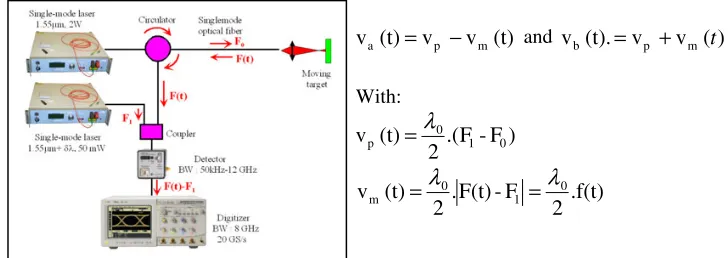
A single mode laser source (frequency F0 or wavelengthλ0) lights a moving target (Fig. 1). The
backreflected light (F(t)=F0.[1+2.v(t)/c]), frequency modulated by the target velocity v(t), is mixed
with a part of the laser source light. We thus get beats versus time at the frequency f(t) (c being the speed of light in vacuum).
f(t)=F(t)−F0=F0.
2·v(t)
c or v(t)=
λ0
2f(t)
Fig. 1. PDV principle. Laser source (IR, CW), Michelson interferometer (all fiber) with the moving target as a
mirror on a leg, detector and recorded signal. Each time the target moves ofλ0/2, the digitizer records one beat.
Count the number of beats per second then allows knowing the velocity versus time: this task is achieved thanks to short time Fourier transform-like processes.
(t)
v
v
(t)
v
a=
p−
m andv
b(t).
=
v
p+
v
m(
t
)
With:
)
F
-F
.(
2
(t)
v
0 1 0p
λ
=
.f(t)
2
F
-F(t)
.
2
(t)
v
0 1 0 mλ
λ
=
=
Fig. 2. Two-laser setup (CW IR lasers, circulator, singlemode fiber, detector, digitizer, 4 channels).
With an infrared erbium laser (λ0 =1.55μm) and few km/s velocities, f(t) is in the few GHz range. Thus, for a 5 km/s velocity, it is necessary to have a 6.5 GHz bandwidth (detector+digitizer). Fur-thermore, according to the Shannon rule, the sampling rate will be at least 13 GS/s (20 GS/s will be suitable). To extract the velocity law we apply a short time Fourier transform with a Hamming windows (width: 25 to 50 ns) to the raw signal, which gives us a spectrogram (x-time, y-velocity, z-power); the searched velocity is obtained by following the local track of maximum power, versus time. To increase this 5 km/s velocity limit, we modified the basic setup by adding a frequency-shifted second laser (frequency F1). Thus, instead of getting beats between F(t) and F0, we get beats between F(t) and F1. The frequency difference F1−F0 (we call it, pivot frequency) is adjustable before shot (between−1 GHz and+6.5 GHz i.e.−0.7 km/s and+5 km/s). With a frequency shift exactly equal to the equipment bandwidth, one doubled the velocity range: 10 km/s instead of 5 km/s. There are two velocity solutions va(t) and vb(t), but only one is physical (vmis the measured velocity).
With such a device it is then possible to observe the apparent velocity of a NM overdriven detona-tion which is around 10 km/s (=7.5 km/s.n0; n0=1.368: NM refractive index @1.55μm). In 2010 we got an 11 GHz bandwidth chain which therefore allowed us to measure up to 17 km/s (=2∗11∗1.55/2). The sampling rate is 50 GS/s. The main CW laser delivers 2 W and the second one 50 mW @1.55μm. Each one is split in four equivalent channels (400 mW and 10 mW/channel). The associated veloc-ity uncertainty (+/−5 m/s) is mainly due to the velocity quantization depending on the Hamming windows width (50 ns) multiplied by the zero padding extension (x3) i.e. 150 ns.
3 Experimental setup
Table 2. List of shots.
Shot Device NM height Detonation PDV fibers (end of line) & probe OZ Pivot Velocity (Fig. 3) behavior (+also 3 piezo probes)
mm singlemode multimode OZ m/s
SMF28 GI62.5 HCP105
FIM 4 A 600 Steady 2 2 0 0 +5111
FIM 1 B 80 Non-Steady 2 2 0 0 +4089
FIM 5 B 80 Non-Steady 2 3 2 1 −219/+8947
FIM 3 C 80 SDT 1 2 0 1 0/ +6259
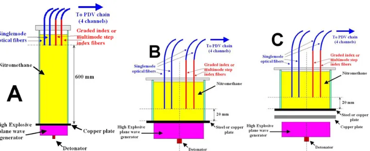
2007 we decided to apply this idea and we built a cylindrical aquarium made of glass: diameter 100 mm, height 80 mm (excepted for shot FIM 2: 650 mm) ended by a metallic plate (steel or copper) and filled with NM. We put a high explosive plane wave generator (diameter 100 mm) under it. Then we submerged, vertically in the NM, 4 to 7 PDV bared optical fibers.
Their ends are set at different distances over the bottom plate (between 15 and 20 mm, and up to 600 mm for the FIM 2 shot). Depending on the shot, there are 3 kinds of submerged bare optical fibers (Table 1).
Indeed, the last two types, theoretically, don’t suit PDV setup since it normally requires singlemode fibers, but the optical path is quite not affected by them (no significant phase information is lost), especially because their lengths are kept short (less than 1 m). They are then connected to a 40 m single mode SMF28 fiber plugged on the PDV velocimeter. The reason of their use relied upon the discovery of their behaviors in such environment and upon the fact that their core diameters and their numerical apertures were bigger than those of the SMF28, thus helping the collection of back reflected light. In this manner, results were satisfying over the four shots we achieved (Table 2).
4 Experimental results
4.1 Shot FIM4 – Steady detonation
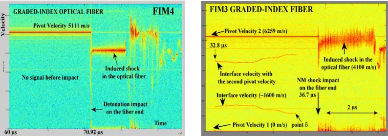
With this experimental configuration (Fig. 3A) we are sure that the detonation is steady, at least 100 mm before hitting fibers ends. The four fibers are set on the top of the setup and submersed vertically, 20 and 30 mm in the NM, perpendicular to the detonation front. Spectrogram is presented in Fig. 8. On the left half part, we see a single constant signal; it corresponds to the pivot velocity (5111 m/s or 6.58 GHz). We don’t see anything else and especially the steady detonation wave (6300 m/s): it does exist, but it doesn’t reflect any infra-red light coming from the fibers, before striking them. If we were able to see it, it would be set at Vmeasured:
Vmeasured=Vreal·nNM−Vpivot→Vmeasured=6300 m/s.1.368−5111 m/s=3507 m/s (4.52 GHz)
It seems to be in agreement with the Dremin hypothesis: the steady detonation wave surface does not reflect any light [5]. On the right side of each spectrogram, we still see the pivot frequency but strongly attenuated; the frequency F0 doesn’t come anymore from the (destroyed) static end of the fiber, but
Fig. 3. “Steady detonation” device on the scheme A, “non steady detonation” device on the scheme B and and “Shock to Detonation Transition” device on the scheme C. For each shot we used from 4 to 8 channels: with single-mode, graded-index and multimode step index fibers (just in the last meter of each line).
Fig. 4. FIM5 multimode step index fiber spectro-gram.
Fig. 5. FIM5 Zoom of Fig. 4
see a new constant signal (between 71 and 75.65μs) at a lower “displayed” velocity (4160 m/s with the graded-index fiber); this is due to the continuation of the detonation along the fiber, creating a shock-mirror in its core. This signal corresponds to a real velocity Vreal: it is close to the velocity of
the steady detonation wave in NM. We divide the result by the effective refractive index of the fiber (graded-index in this case), because the mirror-target moves in this medium.
Vreal=(Vpivot+Vmeasured/nefffiber→Vreal=(5111 m/s+4160 m/s)/1.4957=6198 m/s
This velocity is confirmed by chronometric values (detonation impact times at different fiber end depths) by which we obtain 6285 m/s.
4.2 Shots FIM1 and FIM5 – Non-steady detonation
Fig. 6. FIM5 OZ probe spectrogram (the pivot ve-locity -219 m/s is really negative but appears posi-tive, due to the FFT folding).
Fig. 7. FIM1-FIM5: x-t diagram (deduced superdetonation velocity from PDV signals: about 9500 m/s).
m/s (refracted index corrected) which remains visible 2.8μs. At this time appears the overdriven deto-nation at 7300 m/s (supposed started as superdetonation in the hot NM, when the interface disappears at 16.1μs: Fig. 6, pointα); Dremin [5] affirms that the surface of the overdriven detonation is like a mirror (reflecting light or image).
Its velocity then decreases and it becomes a classical detonation wave after 4μs which is no more visible as FIM4 shot evidenced it. The deceleration of this overdriven detonation is not stable (2 main parts in the shot FIM5 but 1 part in the shot FIM1). However, in these 2 experiments, we observe decelerations with saw teeth shapes (Fig. 5); it could reveal multiple ignitions in time and spatially, may be due to impurities or air bubbles in the NM. At 18.4μs this overdriven detonation reaches the fiber (Fig. 6), set 25 mm from the bottom. The induced fiber shock wave (“glued” to the overdriven detonation) travels at 6480 m/s (index corrected) equal to the overdriven detonation velocity in NM just before impact.
Knowing the extinctions times (Fig. 6 pointsαandβ) of both, the interface velocity track and the NM shock wave velocity track and also knowing their velocities (to calculate their displacements), enable us to derive the superdetonation abscissae when it starts and when it overtakes the shock wave. We are then able to calculate its eulerian average velocity in the pre-shocked NM: 9500 m/s for FIM1 and 9600 m/s for FIM5.
The different observed signals are summarized in the x-t diagram Fig. 7 and already explained by Chaiken and Dremin [5–8].
4.3 Shot FIM3 – Shock to detonation transition
Unlike the other shots for which the induced pressure in NM was 16 GPa (but non sustained constant pressure), it was 8.5 GPa (sustained constant pressure) for this one (Fig. 3C). To decrease the pressure we moved back the high explosive plane wave generator ended by a thick copper plate. So we were expecting a shock-detonation transition much smoother than the FIM1 or FIM5 ones. In fact, no det-onation happened (Fig. 9). We only observed the interface velocity (copper-NM) but no NM shock wave; however it was indirectly observed (∼4100 m/s) by its time impact on the optical fiber, on piezo probes and with PDV fibers, during the first 200 ns (spread velocity signal).
Fig. 8. FIM4 Graded index optical fiber spectro-gram.
Fig. 9. FIM3 spectrogram.
5 Conclusion
PDV is a powerful tool to measure velocity and observe matter under high dynamic pressure. Study-ing shock physics phenomena within transparent matter has also proven to be possible by usStudy-ing simple bare optical fibers; graded-index and multimode step index fibers as probes but connected to classical singlemode fibers, are more sensitive and deliver better signals than the singlemode fiber as probe. These fibers act first, as a no-contact probe then as an intrusive probe (with a lagrangian mirror), at least with detonation wave-like interfaces. Velocities of both shocks and overdriven detonation lo-cated ahead of and within a fiber submerged in nitromethane have been measured. Results confirm the scenario of the superdetonation; it remains still invisible but both the interface and the shockwave disappearances, demonstrate its presence with an estimated velocity of 9500 m/s. These first tests have to be repeated to confirm our interpretation of the behavior of this liquid explosive, especially in the shock detonation transition.
References
1. O.T. Strand et al, “Velocimetry using Heterodyne Techniques”, 26th International Congress on High Speed Photography and Photonics, Alexandria, VA, September 19-24, 2004.
2. D. Holtkamp, “Survey of optical velocimetry experiments – Application of PDV, A heterodyne velocimeter”, 2006 International conference on Mega gauss Magnetic Field Generation. November 5-10, 2006, Santa Fe, USA-New Mexico.
3. P. Mercier, J. B´enier, A. Azzolina, J.M. Lagrange, D. Partouche ”Photonic Doppler Velocimetry in shock physics experiments” Dymat 2006: 8th International conference on mechanical and physical behaviour of materials under dynamic loading. 11-15 septembre 2006. Dijon. France.
4. D. Goosman, G. Avara, J. Wade, A. Rivera (LLNL), “Optical filters to exclude non-Doppler-shifted light in fast velocimetry”, SPIE vol. 4948, 2003.
5. A. Dremin S. Savrov, A. Andrievskii, Comb. Expl. and Shock Waves, Vol.1, p1,1965 7.
6. D.R. Hardesty, “An investigation of the shock initiation of liquid nitromethane”, Combustion and flame, Vol.27, pp. 229-251, 1976.
7. R. Chaiken, “The kinetic theory of detonation of high explosives”, M.S. Thesis, Polytechnic Inst. Of Brooklyn.