Article
A data-driven approach to classifying wave breaking
in infrared imagery
Daniel Buscombe1,∗, and Roxanne J. Carini2
1 School of Earth & Sustainability, Northern Arizona University, Flagstaff, AZ; [email protected]
2 Applied Physics Laboratory, University of Washington, Seattle, WA; [email protected]
* Correspondence: [email protected]
Abstract: We apply deep convolutional neural networks (CNNs) to estimate wave breaking type from close-range monochrome infrared imagery of the surf zone. Image features are extracted using six popular CNN architectures developed for generic image feature extraction. Logistic regression on these features is then used to classify breaker type. The six CNN-based models are compared without and with augmentation, a process that creates larger training datasets using random image transformations. The simplest model performs optimally, achieving average classification accuracies of 89% and 93%, without and with image augmentation respectively. Without augmentation, average classification accuracies vary substantially with CNN model. With augmentation, sensitivity to model choice is minimized. A class activation analysis reveals the relative importance of image features to a given classification. During its passage, the front face and crest of a spilling breaker are more important than the back face. Whereas for a plunging breaker, the crest and back face of the wave are most important. This suggests that CNN-based models utilize the distinctive ‘streak’ temperature patterns observed on the back face of plunging breakers for classification.
Keywords:wave breaking; remote sensing; surf zone; machine learning
1. Introduction
In the surf zone, the spatio-temporal patterns and dynamics of wave breaking generate nearshore currents and transport sediment, which changes seafloor topography. This, in turn, affects wave transformation processes, spatial gradients in energy dissipation, and nearshore hydrodynamic circulation patterns [1]. This circulation determines the fate of seabed nutrients, contaminants, and pathogens, and asserts control on the seabed and water column as habitats [2]. Numerical modeling of the onset of wave breaking and the amount of energy lost during breaking (dissipation) usually relies on parameterizations such as Thornton and Guza [3] and Duncan [4]. The evolution of individual waves toward breaking is not fully understood [5], and there is no consensus on a method for predicting the statistics of breaking waves [6]. Therefore, detailed observations of wave breaking are needed to develop improved parameterizations of wave transformation and energy dissipation processes across the surf zone.
Breaking waves are classified into discrete classes, namely collapsing, surging, plunging, and spilling [7]. Plunging (when the wave crest curls forward and abruptly impinges the water surface) and spilling (when an aerated roller cascades down the front face of the wave) are the most common breaker types on open coastlines and sandy beaches. Spilling and plunging breakers have different rates of energy dissipation [8]. Therefore, a robust, fully automated, objective approach to classifying breaker type and other wave properties from remote sensing data would be an extremely valuable tool for studying surf zone energy budgets. Thermal infrared (IR) imagery has been used to study deep-water wave breaking [9], microscale breaking [10], and surf zone wave breaking [11] because it is relatively insensitive to reflected light from the sun and sensitive to the subtle temperature
Entropy2016,xx, x; doi:10.3390/—— www.mdpi.com/journal/entropy
difference between relatively warm active foam (the foam produced during active breaking) and relatively cool residual foam (the foam left behind in the wake of a breaking wave). Additionally, distinctive streaky temperature patterns have been observed on the back face of plunging waves in IR imagery [12,13]. However, to our knowledge, no attempt has been made to either mechanistically relate the energy content of wave breaking to specific IR temperature patterns, or to harness those IR textures to infer statistical descriptors of spilling and plunging breakers. Here, we successfully attempt the latter.
In recent years, while applied machine learning technologies have developed at an unprecedented pace [14], there has been a concomitant interest in their application to imagery of coastlines for academic research [15–17], beach monitoring, and for leisure purposes. Indeed, the recent proliferation in coastal imaging systems is driven in part by the expectation that such artificially intelligent technologies will make data-driven observations of surf zone hydrodynamics feasible. A specific class of machine learning algorithms called deep convolutional neural networks (CNNs, also known as DCNNs or Convnets), has been shown to produce state-of-the-art performance for a variety of image recognition and classification tasks [e.g.,18–21]. A major reputed advantage of deep learning over conventional machine learning is that it does not require manual feature selection and extraction. These practices select or transform image data to make them more amenable to a specific algorithm or to reduce model overfitting, thereby increasing model generality. Another attractive aspect of deep learning models is that they can be used as generic feature extractors by initializing each model “neuron” with a set of weights and biases learned from a different dataset, such as Imagenet [22], a library of millions of labeled generic images. This widespread practice is called ‘transfer learning’ [23] and makes model training considerably faster.
Here, we employ CNN models on a training set of IR images of breaking or near-breaking surf zone waves to create a function that estimates wave breaking type from an arbitrary single image. Feature extraction is automatic, and predictions are made based on image texture related to small-scale spatial patterns in sea surface temperature. The success of the classification is a test of how well generic CNN models, initialized with weights learned from a different dataset and a different set of classes, extract geophysically relevant information from imagery.
2. Materials & Methods
2.1. Field site and instrumentation
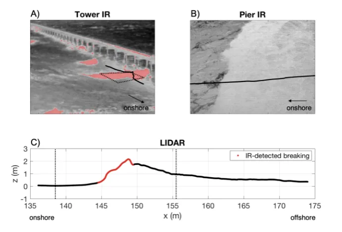
Observations of breaking waves in the outer surf zone were collected using a thermal IR camera during a field campaign, 7-8 November 2016, at the US Army Corps of Engineers (USACE) Field Research Facility (FRF) in Duck, North Carolina, United States. A DRS UC640-17 long-wavelength (8-14µm), uncooled VOx Microbolometer IR camera was mounted to the FRF pier and stabilized by
four guy lines attached to the pier railings. This camera viewed the sea surface at 45◦incidence angle and collected data continuously at 10 Hz. A continuously operating Riegl VZ-400 LIDAR (LIght Detection and Ranging), with ≤1cm accuracy measured the sea surface elevation across a profile intersecting the field of view of the IR camera. An example IR image of a spilling breaker is shown in Figure1B. For context, Figure1A shows a surf zone-scale view of the same breaker, and Figure
1C displays the LIDAR profile of the breaker. In this study, 10.5 hours of data were used, during which time wave height and period both varied significantly, from 0 to 5.94 m and 2.32 to 19.36 s, respectively, measured using the LIDAR profiles.
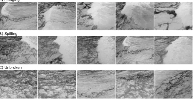
streak pattern on the back face of the wave (Figures2A), whereas spilling breakers are identified by more unorganized texture on the back face of the wave (Figures2B).
Figure 2.Example IR images of the three categorical wave classes: (A) plunging, (B) spilling, and (C) unbroken waves. The back face of a spilling breaker exhibits a unorganized texture whereas that of a plunging breaker is characterized by an organized streak pattern.
2.2. Model for discrete classification of breaker type
A supervised machine learning approach estimates a function f that maps inputsx(a training set of IR images of waves) to corresponding outputs y (labels of wave breaker class) such that y = f(x). This function is then used to make predictions on unlabeled data. Several open-source CNN architectures have been designed to recognize objects and features in non-specific photographic imagery [24]. Among numerous suitable, popular, state-of-the-art and open-source frameworks for whole-image classification using CNNs, we choose MobilenetV2 [25], Xception [26], Resnet50 [27], InceptionV3 [28], Inception-ResnetV2 [29] and VGG19 [19] (in increasing order of number of tunable model parameters). These CNNs automatically generate a hierarchy of features that are learned from input data using a general-purpose procedure. This procedure applies a set of convolution filters to extract local features and spatially shares the parameters of each filter. The weights of the filters in each layer are learned using back-propagation [14], an optimization process that minimizes the error between the output produced by the CNN and the ground-truth label. Each model is implemented using the TensorFlow symbolic math library [30]. Logistic regression on the extracted features is then used for discrete classification. Letxbe the features extracted from the last pooling layer of the CNN. To handle ambiguity, the most probable wave breaker class is found by solving,
y= f(x) =argmaxC
c=1
p(y=c|x), (1)
whereCis a vector of possible classes (unbroken, spilling, or plunging). Equation (1) is computed by transformingxinto a discrete probability distribution over thek=3 possible classes using multinomial logistic regression, known in the field of machine learning as the softmax function [31]:
p(y=c|x) = e x
∑k k=1ex
. (2)
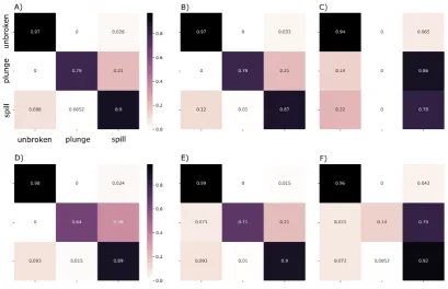
Table 1. CNN classification results. Rank-1 and F1 scores for each of 6 models without (and with) image augmentation.
Model Rank-1 Score F1 Score
Unbroken Plunging Spilling MobilenetV2 0.95 (0.94) 0.97 (0.96) 0.85 (0.95) 0.90 (0.89) Xception 0.94 (0.92) 0.96 (0.95) 0.81 (0.93) 0.88 (0.86) Resnet-50 0.87 (0.78) 0.92 (0.87) 0.0 (0.6) 0.76 (0.68) InceptionV3 0.95 (0.94) 0.97 (0.96) 0.69 (0.95) 0.9 (0.9) InceptionResnetV3 0.96 (0.93) 0.98 (0.95) 0.77 (0.95) 0.92 (0.89) VGG19 0.93 (0.90) 0.96 (0.94) 0.24 (0.86) 0.88 (0.83)
equivalent outputs from a simple generative approach, whereby the posterior label probabilities are found using Bayes’ theorem:
p(y|x) = p(x|y)p(y)
p(x) ; p(x) =
∑
p(x|y)p(y). (3) The inferior skill of this so-called ‘naive Bayes’ approach is likely due to the extracted image features not contributing independently to the probability of a given classification (i.e., the features are correlated, violating the assumptions of the model). Models are trained without and with image augmentation. Augmentation is implemented using the following random changes to the images: 1) shifts in either or both image dimensions of up to 10%; 2) rotations up to±10 degrees; 3) shear in either axis up to 5 degrees; and 4) zoom up to 20% by image area. Image vertical and horizontal flipping is another common strategy employed to augment training datasets, but it was not employed here because image textures are anisotropic (i.e., the direction of wave propagation is important to image texture). All classified images are randomly split into a training set and a testing set. The data used to train the CNN models consists of 5455 (7455) images of unbroken waves, 138 (2138) images of plunging breakers, and 1904 (3904) images of spilling breakers without (with) augmentation. The testing data consists of 1820 images of unbroken waves, 47 images of plunging breakers, and 636 images of spilling breakers. Each image is cropped to square then reduced to 299×299 pixels, for computational efficiency.3. Results
To assess classification performance, we compare the automated CNN classifications against the test dataset (Table1). Based on Rank-1 scores, which is the percentage of samples for which the model correctly estimates wave breaker class, there is little difference between MobilenetV2, InceptionV3, and Inception-ResnetV2 (in order of increasing model complexity). Resnet-50 is the worst performing model, without and with image augmentation. The general prediction skill of the model for individual classes is assessed using an F1 score, which is an equal weighting of the recall and precision. Precision and recall are standard accuracy metrics employed when the number of observations belonging to one class (plunging) is significantly lower than those belonging to the other classes (spilling and unbroken), which is the case here. Precision is the proportion of positive identifications that are correct (a precision of 1 means there are no false positives), and recall is the proportion of actual positives identified correctly (a recall of 1 means there are no false negatives). F1 scores (Table1) reveal greater differences between models and highlight the prediction improvement achieved using image augmentation.
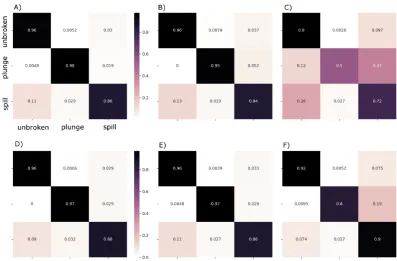
for models trained without (Figure3) and with (Figure4) augmentation shows that the latter ensures individual class predictions have errors of less than 50%, regardless of CNN model used. All augmented models with the exception of Resnet-50 are accurate to within 20% for all classes. Without augmentation, misclassifications are much more likely.
Figure 3.Confusion matrices for models training without image augmentation: A) MobilenetV2; B) Xception; C) Resnet-50; D) InceptionV3; E) Inception-ResnetV2; F) VGG19. For each confusion matrix, the abscissa represents estimated and the ordinate represents true.
4. Discussion & Conclusions
Transfer learning —that is, using a deep neural network with weights learned using another dataset —as a generic feature extractor, combined with a simple logistic regression classifier, was sufficient for estimating wave breaker class from IR images of the surf zone with high accuracy. For most models, however, image augmentation improved classification performance. This supports the general consensus among machine learning experts that CNNs require large datasets and performance increase is to be expected with more data [32]. This holds even if the classical notion of data information content is challenged by the enormous amount of redundancy in the augmented data. It is widely known that effective use of logistic regression requires large sample sizes [31], hence the importance of augmentation. Augmentation would also further aid end-to-end model training that optimizes the model used as a feature extractor for the specific data set.
Figure 4. Confusion matrices for models training with image augmentation: A) MobilenetV2; B) Xception; C) Resnet-50; D) InceptionV3; E) Inception-ResnetV2; F) VGG19. For each confusion matrix, the abscissa represents estimated and the ordinate represents true.
accuracy (Table 1). It will be interesting to observe how well these observations hold for other geophysical classification problems.
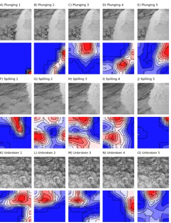
The global average pooling (GAP) layers in modern CNN feature extractors are crucial to minimize overfitting by reducing the total number of parameters in the model. Further, Zhouet al. [33] and subsequent studies have demonstrated that CNNs with GAP layers that have been trained for a classification task can also be used for object localization. In a conventional sense, this is where an object is in the image. In the present case, we can use this technique to indicate how important each location is with respect to the wave breaker class prediction. The localization is expressed as a ‘class activation map’, where relatively large values indicate regions that are relatively important for the CNN to perform the classification task. We implemented the method of Zhouet al.[33] on five sequential example images of each wave breaker class. Scrutiny of the results in Figure5reveals that different features are important, depending on the type of wave or breaker and also on the stage in its temporal evolution. During the passage of a spilling breaker, regions of the image near the wave crest and on the front face of the wave (Figure 5A-5E) are most important. For a plunging breaker, (Figure5F-5J), regions of the image near the wave crest and on the back face of the wave are most important. This supports a hypothesis that the CNN is picking up on the distinctive ‘streak’ temperature patterns observed on the back face of plunging breakers [12,13]. Therefore we argue that not only does the network generally make the correct classification, it also assigns those classes for the right reasons. Such visualization techniques could therefore lead to improved mechanistic understanding of the hydrodynamics or thermodynamics of wave breaking.
and plunging, those waves whose IR signature is not clearly spilling or plunging pose a challenge to both the DCNN and the eye. Future work to incorporate knowledge of sequential classifications into the CNN algorithm may therefore help to define additional classes, such as the transition between onset and steady state breaking. The ratio of prediction probabilities of spilling and plunging waves may also be a useful metric to determine where a given wave exists on the continuum of breaker type. We have presented a technique that may be applied on imagery representing a small spatial footprint of just a few square meters. Therefore, it seems likely that data-driven approaches such as this might be used to identify specific waves in a field of breaking waves by analyzing small regions of imagery with large spatial footprints of thousands of square meters, which would open new research avenues. Another potential next step in application of CNN techniques to IR imagery in the surf zone is image segmentation, which involves classifying every pixel in an image [23,34,35]. Of particular interest would be the spatial extent of active and passive foam, as well as streaks and other thermal patterns, which may be useful to estimating wave energy dissipation.
Acknowledgments:RJC thanks Kate Brodie, Nick Spore, Jason Pipes, and the entire USACE FRF staff for field support; Dan Clark, Phil Colosimo, and John Mower for IR camera hardware and software development; and Melissa Moulton, Seth Zippel, and Meg Palmsten for fieldwork help. RJC was funded by NSF grant number 1736389 and ONR grant number N000141010932. This study is fully reproducible using data and code available athttps://github.com/dbuscombe-usgs/IR_waveclass.
Conflicts of Interest:The authors declare no conflict of interest.
Bibliography
1. MacMahan, J.H.; Thornton, E.B.; Reniers, A.J. Rip current review. Coast. Eng.2006,53, 191–208.
2. Defeo, O.; McLachlan, A.; Schoeman, D.S.; Schlacher, T.A.; Dugan, J.; Jones, A.; Lastra, M.; Scapini, F. Threats to sandy beach ecosystems: a review. Estuar. Coast. Shelf S2009,81, 1–12.
3. Thornton, E.B.; Guza, R. Transformation of wave height distribution. J. Geophys. Res. Oceans1983, 88, 5925–5938.
4. Duncan, J. An experimental investigation of breaking waves produced by a towed hydrofoil. Proc. R. Soc. Lond. A1981,377, 331–348.
5. Banner, M.; Peregrine, D. Wave breaking in deep water. Annu. Rev. Fluid Mech.1993,25, 373–397. 6. Filipot, J.F.; Ardhuin, F.; Babanin, A.V. A unified deep-to-shallow water wave-breaking probability
parameterization. J. Geophys. Res. Oceans2010,115.
7. Basco, D.R. A qualitative description of wave breaking. J. Waterw. Port Coast.1985,111, 171–188. 8. Iafrati, A. Energy dissipation mechanisms in wave breaking processes: spilling and highly aerated
plunging breaking events. J. Geophys. Res. Oceans2011,116.
9. Jessup, A.; Zappa, C.; Loewen, M.; Hesany, V. Infrared remote sensing of breaking waves. Nature1997, 385, 52.
10. Jessup, A.; Zappa, C.J.; Yeh, H. Defining and quantifying microscale wave breaking with infrared imagery. J. Geophys. Res. Oceans1997,102, 23145–23153.
11. Carini, R.J.; Chickadel, C.C.; Jessup, A.T.; Thomson, J. Estimating wave energy dissipation in the surf zone using thermal infrared imagery. J. Geophys. Res. Oceans2015,120, 3937–3957.
12. Watanabe, Y.; Mori, N. Infrared measurements of surface renewal and subsurface vortices in nearshore breaking waves.J. Geophys. Res. Oceans2008,113.
13. Huang, Z.C.; Hwang, K.S. Measurements of surface thermal structure, kinematics, and turbulence of a large-scale solitary breaking wave using infrared imaging techniques. Coastal Engineering2015, 96, 132–147.
14. Goodfellow, I.; Bengio, Y.; Courville, A.; Bengio, Y.Deep Learning; Vol. 1, MIT press Cambridge, 2016. 15. Holman, R.; Haller, M.C. Remote sensing of the nearshore. Annu. Rev. Mar. Sci.2013,5, 95–113.
16. Baldock, T.E.; Moura, T.; Power, H.E. Video-Based Remote Sensing of Surf Zone Conditions. IEEE Potentials2017,36, 35–41.
18. Krizhevsky, A.; Sutskever, I.; Hinton, G.E. Imagenet classification with deep convolutional neural networks. Adv. Neur. In., 2012, pp. 1097–1105.
19. Simonyan, K.; Zisserman, A. Very deep convolutional networks for large-scale image recognition. arXiv preprint arXiv:1409.15562014.
20. Howard, A.G.; Zhu, M.; Chen, B.; Kalenichenko, D.; Wang, W.; Weyand, T.; Andreetto, M.; Adam, H. Mobilenets: Efficient convolutional neural networks for mobile vision applications. arXiv preprint arXiv:1704.048612017.
21. Gu, J.; Wang, Z.; Kuen, J.; Ma, L.; Shahroudy, A.; Shuai, B.; Liu, T.; Wang, X.; Wang, G.; Cai, J.; Chen, T. Recent advances in convolutional neural networks. Pattern Recogn.2017,77, 354–377.
22. Deng, J.; Dong, W.; Socher, R.; Li, L.J.; Li, K.; Fei-Fei, L. Imagenet: A large-scale hierarchical image database. Proc. CVPR IEEE. IEEE, 2009, pp. 248–255.
23. Buscombe, D.; Ritchie, A. Landscape classification with deep neural networks. Geosciences2018,8, 244. 24. Russakovsky, O.; Deng, J.; Su, H.; Krause, J.; Satheesh, S.; Ma, S.; Huang, Z.; Karpathy, A.; Khosla, A.;
Bernstein, M.; others. Imagenet large scale visual recognition challenge. Int. J. Comput. Vision2015, 115, 211–252.
25. Sandler, M.; Howard, A.; Zhu, M.; Zhmoginov, A.; Chen, L.C. MobileNetV2: Inverted Residuals and Linear Bottlenecks. arXiv preprint arXiv:1801.043812018.
26. Chollet, F. Xception: Deep Learning With Depthwise Separable Convolutions. Proc. CVPR IEEE, 2017, pp. 1251–1258.
27. He, K.; Zhang, X.; Ren, S.; Sun, J. Deep residual learning for image recognition. Proc. CVPR IEEE, 2016, pp. 770–778.
28. Szegedy, C.; Vanhoucke, V.; Ioffe, S.; Shlens, J.; Wojna, Z. Rethinking the inception architecture for computer vision. Proc. CVPR IEEE, 2016, pp. 2818–2826.
29. Szegedy, C.; Ioffe, S.; Vanhoucke, V.; Alemi, A.A. Inception-v4, Inception-Resnet and the impact of residual connections on learning. AAAI, 2017, Vol. 4, p. 12.
30. Abadi, M.; Agarwal, A.; Barham, P.; Brevdo, E.; Chen, Z.; Citro, C.; Corrado, G.S.; Davis, A.; Dean, J.; Devin, M.; others. Tensorflow: Large-scale machine learning on heterogeneous distributed systems. arXiv preprint arXiv:1603.044672016.
31. Murphy, K.Machine learning: A probabilistic perspective; MIT press Cambridge, 2012. 32. LeCun, Y.; Bengio, Y.; Hinton, G. Deep learning. Nature2015,521, 436.
33. Zhou, B.; Khosla, A.; Lapedriza, A.; Oliva, A.; Torralba, A. Learning deep features for discriminative localization. Proc. CVPR IEEE, 2016, pp. 2921–2929.
34. Long, J.; Shelhamer, E.; Darrell, T. Fully convolutional networks for semantic segmentation. Proc. CVPR IEEE, 2015, pp. 3431–3440.
35. Fu, G.; Liu, C.; Zhou, R.; Sun, T.; Zhang, Q. Classification for high resolution remote sensing imagery using a fully convolutional network.Remote Sens.2017,9, 498.
c