Trust-region based methods for unconstrained global optimization

TRUST-REGION BASED METHODS FOR UNCONSTRAINED GLOBAL OPTIMIZATION

KERK LEE CHANG

A thesis submitted in fulfilment of the requirements for the award of the degree of

Doctor of Philosophy

Faculty of Science Universiti Teknlogi Malaysia

DEDICATION

ACKNOWLEDGEMENT

First of all, I would like to express my gratitude to my thesis supervisor, Professor Madya Dr Rohanin Bt. Ahmad for her guidance and support in completing my thesis. Her encouragement, patience, motivation enthusiasm, and immense knowledge motivated me to finish this thesis. She gives me a lot of valuable advice and guidance when I encountered the challenges. Her supervision inspired me a lot.

I am also grateful and very appreciative of the encouragement, support, love and care from my family and friends. Thanks for always being there for me during the good and the bad. They have always been behind me and pushed me to be the best that I can do. Their caring and inspiration were driving me to finish this thesis.

ABSTRACT

ABSTRAK

TABLE OF CONTENTS

CHAPTER TITLE PAGE

DECLARATION ii

DEDICATION iii

ACKNOWLEDGEMENT iv

ABSTRACT v

ABSTRAK vi

TABLE OF CONTENTS vii

LIST OF TABLES xi

LIST OF FIGURES xii

LIST OF ABBREVIATION xiv

LIST OF SYMBOLS xvi

LIST OF APPENDICES xx

1 INTRODUCTION

1.0 Overview

1.1 Introduction

1.2 Background of Problems 1.3 Statements of Problems 1.4 Research Questions 1.5 Objectives of the Study 1.6 Scope of the Study 1.7 Significance of the Study 1.8 Research Outline

1

1 4 9 10 11 11 12 12

2 LITERATURE REVIEW

2.0 Overview

2.1 Introduction to Optimization

2.2 Nonlinear Optimization 2.3 Local Optimization (LO)

2.3.1 Newton’s Method 2.3.2 Gradient Descent

2.3.3 Quasi-Newton’s Method

2.4 Global Optimization (GO)

2.4.1 Homotopy Based Methods 2.4.2 Interval-based Methods

2.5 Discussion on Techniques Used to Replace IVT 2.6 Conclusion 17 18 19 21 21 22 23 25 31 34

3 RESEARCH METHODOLOGY

3.0 Overview

3.1 Research Design and Procedure 3.2 Improving HSPM

3.2.1 Improve HSPM 3.2.2 Extention of KRTI 3.3 Homotopy

3.4 Poincaré-Miranda Theorem (PMT) 3.5 Theoretical Analysis

3.5.1 Aysmptotic Algorithm Analysis

3.5.2 Descent Property 3.5.3 Convexity

3.5.4 Zangwill’s Global Convergence Theorem 3.6 Summary 37 37 42 43 44 44 46 47 47 50 51 52 53

4 DEVELOPMENT OF KRTI

4.0 Overview 4.1 Introduction 4.2 Analysis of HSPM

4.3 The Improved Algorithm from HSPM: KRTI 4.4 Convexity of KRTI

4.5 Global Convergence

4.6 Numerical Experiments 4.6.1 Test Function 4.6.2 Numerical Results

4.6.3 Discussion and Summary 4.7 Time Complexity of KRTI

4.8 Conclusion 74 75 87 89 89 93

5 EXTENSION OF KRTI TO MULTIDIMENSIONAL

PROBLEMS

5.0 Overview 5.1 Introduction

5.2 KRTR

5.3 Convexity of KRTR

5.4 Globally Convergence of KRTR 5.5 Gallery of Test Functions

5.5.1 Standard Test Functions 5.5.2 Low Success Rate’s Functions 5.6 Results and Discussion

5.6.1 Numerical Reults of KRTR

5.6.2 Simulation of KRTR for Low Success Rate Cases

5.7 Discussion and Conclusion 5.8 Summary 95 95 99 100 103 105 105 117 121 122 125 127 131

6 SUPERIORITY OF DEVELOPED ALGORITHMS

AGAINST HOPE

6.0 Overview

6.1 Introduction of HOPE

6.2 KRTR

6.3 The Comparison of Simulation of KRTI, KRTR and HOPE

6.3.1 KRTR versus HOPE 6.3.2 KRTI versus HOPE

6.4 Time Complexity Analysis of HOPE and KRTR 6.5 Analysis of HOPE and KRTR

6.6 Conclusion

145 149 151

7 SUMMARY AND CONCLUSION

7.0 Overview

7.1 Summary of Study 7.2 Contribution of the Study 7.3 Conclusion

7.4 Suggestions for Future Work

153 153 155 157 159

REFERENCES 161

LIST OF TABLES

TABLE NO. TITLE PAGE

4.1 Numerical result of Dixon function. 58

4.2 Numerical result of Dixon-Szego function

computed with good parameter s. 63

4.3 Numerical result of Dixon-Szego function

computed with poor parameter s. 64

4.4 Details of Test Functions. 85

4.5 Auxiliary functions used by KRTI. 86

4.6 Relative error between the approximate solution and the exact solution of 15 Test Functions obtained by KRTI.

87

4.7 Record of Successes and failures in locating

global minimizer of 15 TFs. 88

4.8 Success rates and failure rates. 89

4.9 CPU time of HSPM and KRTI. 90

5.1 Numerical results of KRTR. 122

5.2 Numerical results of low success rate in locating

global solution problems of KRTR. 126

5.3 Numerical results of TF 9 with different step

sizes. 129

5.4 Numerical results of TF 4 with different step

sizes 129

6.1 Numerical result of HOPE obtained by Dunlavy

and Leary. 141

6.2 Numerical results of HOPE versus KRTR. 142

6.3 Numerical results of KRTI by using N-modal

LIST OF FIGURES

FIGURE NO. TITLE PAGE

1.1 Classes of optimization problem. 2

1.2 3D plot of the Function (1.1). 5

1.3 Contour plot of theFunction (1.1). 6

3.1 The operational framework of the research. 40 3.2 (a) Stage 1 of the theoretical framework of the research. 41 3.2 (b) Stage 2 of the theoretical framework of the research. 42

4.1 Dixon function. 59

4.2 Dixon-Szego Function varies from 0 to 1. 60 4.3 Derivative values of Dixon-Szego function for s0.2

and 0.3 respectively.

62

4.4 TF 1. 75

4.5 TF 2. 76

4.6 TF 3. 77

4.7 TF 4. 77

4.8 TF 5. 78

4.9 TF 6. 79

4.10 TF 7. 79

4.11 TF 8. 80

4.12 TF 9. 81

4.13 TF 10. 81

4.14 TF 11. 82

4.15 TF 12. 83

4.16 TF 13. 83

4.17 TF 14. 84

4.18 TF 15. 85

4.19 Time complexity of HSPM. 91

5.1 Ackley’s function. 106

5.2 Hyper-ellipsoid function. 106

5.3 Sum of the different power function. 107

5.4 Extended Easom’s function. 108

5.5 Equality-constrained function. 108

5.6 Griewank’s function. 109

5.7 Michaelwicz’s function. 110

5.8 Rastrigin’s function. 111

5.9 Rosenbrock’s function. 111

5.10 Schwefel’s function. 112

5.11 Six-hump Camel Back function. 113

5.12 Xin-She Yang’s function. 114

5.13 Standing-wave function. 114

5.14 Yang’s Multimodal function. 115

5.15 Zakharov’s function. 116

5.16 Overall Success Rate (Gavana, 2016) 117

5.17 Damavandi function. 118

5.18 Trefethen function. 119

5.19 RosenbrockModified function 120

5.20 Salomon function 121

5.21 Basins of attraction. 128

6.1 The flow chart of the development history of KRTR. 136

6.2 Freudenstein and Roth function. 137

6.3 Jennrich and Sampson function. 138

6.4 N-modal Sine Function and its corresponding auxiliary

functions with

N



10, 20,30, 40,50,60

respectively.

140

6.5 Results of 1000 runs of HOPE on Function (6.4) (solid lines) and Function (6.5) (dashed lines) taken from Dunlavy and Leary (2005).

144

6.6 Time complexity of HOPE. 146

LIST OF ABBREVIATIONS

DE - Differential Evolution

FR - Failure Rate

Freu - Freudenstein and Roth Function

GO - Global Optimization

GOM - Global Optimization Methods

HOM - Homotopy Optimization Method

HOPE - Homotopy Optimization with Perturbations and Ensembles

HSPM - Homotopy 2-Step Predictor-corrector Method

HSPMI - Improved HSPM

HSPMIE - Extended HSPMI

IP - Interger Programming

IVT - Intermediate Value Theorem

Jenn - Jennrich and Sampson Function KRTI - Kerk and Rohanin’s Trusted Interval KRTR - Kerk and Rohanin’s Trusted Region

LO - Local Optimization

LOM - Local Optimization Method

M8 - Mathematica version 8.0

max - Maximize/ maximum

min - Minimize/ minimum

MILP - Mixed Integer Linear Programming

NA - Numerical Analysis

NM - Nelder Mead

NP - Nonlinear programming

N-S - N-modal Sine Function

PCH - Predictor-Corrector Halley's method

QN - Quasi-Newton

RS - Random Search

ROA - Region of Attraction

SA - Simulated Annealing

SR - Success Rate

TF - Test Function

TI - Trusted Interval

LIST OF SYMBOLS

C_ - A collection of convex sets

Z - A continuous function

K - A corresponding value of c over function f, constant

( )

HOPE x

,

( )

HSPM x

,

( )

Z x

,

Z y

( )

- A function

N - A neighbourhood of an extremizer/ a point

D - A nonempty, closed set

p, q, x_n, x_n1,

m x , x_m₁

- A point

l - A solution set

c - _{A value/ element in between interval}

_{[ , ]}

_{a b}

A - An algorithm

( )

g x

- Auxiliary function

O - Big oh notation, constant

 - Big theta notation

1 2

[ ,x x ],

1 2

[ ,y y ],

[ , ]

a b

,

[ , ]

c d

,

x I , I_y

- Closed interval

L,P - Constant

k - Constant, number of iteration

( ) i

c x - Constrained function

Maximum number of iteration k

h - Convergence-control parameter

C, S₁, S₂ - Convex set

f - Currently smallest value of function f

 - Derivative

x

f - Partial derivative of function f with respect to x

y

f - Partial derivative of function f with respect to y

▄ - End of proof

*

x - Extremizer

*

f

,

y

*

- Extremum/ global minimum

( )

f x

- Function f or target function

(1)

x

- Global solution

( )

t x

- Generic homotopy function

n

g - Gradient or first derivative of function f

( )_n

F x ,

H x

( )

- Hessian function

( , )

H x



,

( , , )

H x y



- Homotopy function

 - Homotopy parameter

i

subinterval - i number of subintervals fulfilled the condition by

HSPM/ KRTI within the. interval

[ , ]

a b

 - Infinitesimal change of the dependent variable, error, stopping criterion

 - Infinitesimal increment of the independent variable

0

x ,

x

0,

{ , }x y_{i i} ,

( ,x y_{k k})

- Initial guess

,0

i

x - Initial point, randomly select from subinterval_i

l, ₀ - Initial value for homotopy loop

n

B - Inverse matrix

(k 1) j

x  - jth point in the ensemble at the start of iteration k

k

subinterval - k number of subintervals after the filteration

 - Least upper bound for A

I - Left hand side of interval n

I

a, f R, R

f - Lower bound of an interval

n

a - _{Lower bound of interval}

n I

i

a - Lower bound of subinterval_i

max

c - Maximum number of points in an ensemble

M - _{Maximum number of}

i

subinterval , constant

m

subinterval - m number of subintervals fulfilled the condition by

KRTR on x-axis.

n, j, i, k - Number of iteration

c - Number of perturbations generated of each point in the ensemble

(k 1)

c

 - Number of points in the ensemble at the beginning of iteration k

n

subinterval - n number of subintervals fulfilled the condition by

KRTR on y-axis.

( )

F x

- Objective function



_{- Performing a single steepest descent step}



- Perturbation

( ) ,0 k j

x - Point found by minimization starting at x(_jk1)

( ) , k j i

x - Point found by minimization starting at the ith

perturbation of x(jk 1)



R - Real number

n

R - Real coordinate space of n dimensions,

I - Right hand side of interval In 2



- Second derivative

( ( )),

O g n

( ( ))

O h n

,

- Set of complexity function

n - Size input, number of iteration, constant

, ( )k

, , t,

s, st, sx, sy

- Step length/ step size

k

x

- Solution computed by local search



a b1, 1

 

 a bn, n



- Sub-region

( ) HOPE

T n - Time complexity of HOPE

( ) HSPM

T n - Time complexity of HSPM

( ) KRTI

T n - Time complexity of KRTI

( ) KRTR

T n - Time complexity of KRTR

( )

T x

- Tunnelling function

2

c

- Twice-continuously differentiable

b, f L, fL - Upper bound of an interval

n

b - _{Upper bound of interval}

n I

i

b - _{Upper bound of}

i subinterval

x, y, z, N - Variable

( )k

LIST OF APPENDICES

APPENDIX TITLE PAGE

A KRTI Programming Coded by Mathematica

166

B KRTR Programming Coded by Mathematica 169

CHAPTER 1

INTRODUCTION

1.0 Overview

This chapter provides the definition and brief explanation to give a necessary and clearer understanding of this study. An introduction of optimization is described in Section 1.1. The background, statement, research questions, objectives, scope and significance of the study will be discussed in Section 1.2 to Section 1.7. A research outline is provided in Section 1.8.

1.1 Introduction

Optimization is used widely in our daily life. It is a powerful tool, especially in the engineering field. For instance, it helps engineers to design aircraft with minimum weight and maximum strength, maximize the power output of electrical networks and machinery while minimizing heat generation. Also, optimization has been applied in the economic field to minimize the total transportation cost of shipping x units of products from origin to destination to name a few.

Optimization problems can be classified into several categories as shown in Figure 1.1. Optimization problems can be divided into two main categories which are discrete and continuous optimization. Discrete optimization can be separated into

integer programming and combinatorial optimization. While continuous optimization problems involved nonlinear programming and these problems can be categorized into unconstrained and constrained problem. The optimization problems can be further classified. Details can be referred in Neos (2016).

Figure 1.1: Classes of optimization problem.

Each type of methods which used to solve these problems is a reliable tool in solving optimization problems. For example, the integer programming (IP), a well-known method in optimization that can help to solve an air-crew scheduling problem

(Hoffman and Padberg, 1993). A mixed integer linear programming (MILP) is used to minimize the total control cost consisting of operating and investment cost (Rodrigues et al., 2014). A nonlinear programming (NP) can be used to minimize the size of a tank, and its optimal result helps to explain why soft drink cans are long and thin while storage tanks are short and fat (Shaban et al., 1997).

In general, optimization problems can be viewed as a decision problem that involves finding the "best" solution of the decision variables over all possible

Optimization

Stochastic Deterministic

Continuous

Constrained

Network optimization

Bound constrained

Unconstrained

Local optimization

Global optimization

Discrete

Integer programming

candidates’ solution in the feasible region. By the "best" solution, it can be defined as

the smallest value of the objective function and such a solution is called a minimizer of the objective function over a feasible region. It also can be defined as the biggest value of the objective function and called as a maximizer.

An optimization problem consists of three important elements, which are objective function, constraints and variables. An objective function is needed to minimize or maximize the system. Constraints can comprise of a feasible region that defines limits of performance for the system. Variables used in the system are adjustable to satisfy the constraints (Biegler, 2010).

Today, optimization is a dominant and indispensable decision-making tool. Many industries apply optimization techniques in their daily operation. For example, it is applied in the area of chemistry to minimize the total cost of the heat exchange and used in biology field to predict new designs of movement and behaviours of animals that may yet evolved (Banga, 2008). Minimizing costs is a natural goal to use optimization (Antoniou and Lu, 2007). Besides that, wastage of materials, the way of arranging productions lines machinery, location of warehouses and products storage can also be optimized.

Based on Biegler (2010), optimization is encountered in all facets of chemical engineering from model and process development to process synthesis and design and finally to process operations, control, scheduling and planning. It becomes a major technique to keeps the chemical industry to remain competitive.

type of food which need to be purchased and the constraints are nutritional needs to be satisfied, like total calories, or amount of vitamins, and minerals in the diet.

In physics, a nonlinear multi-objectives technique is used to solve

electromagnetic problem. The objective functions are highest efficiency, lowest cost, and minimum weight of active materials (Duan and Ionel, 2013).

In order to satisfy the requirement from various areas, many methods were established. From Figure 1.1, nonlinear unconstrained optimization can be categorized into local optimization (LO) and global optimization (GO). For example, unconstrained optimization can be used to calibrate a multi-surface-plasticity of a soil constitute model (Yang and Elgamel, 2003).

Existing methods for solving local optimization problem, called local search methods are Newton's method, Golden Section Search method, Steepest descent method to name a few. These methods are usually iterative methods. They will start by initial guesses and stop executing when they found one local solution (Chong and Zak, 2013). While global search methods like Hill Climbing Method, Tunneling

Method, Multi-start method, etc are used to solve global optimization problems.

1.2 Background of Problems

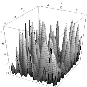
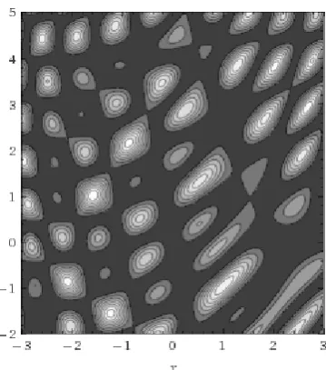
Solving a general unconstrained nonlinear optimization can be very hard, even when the problem is small in size since the feasible region of the problem is not always convex (Guenin et al., 2014). To illustrate the potential difficulty of general unconstrained nonlinear optimization, consider the following model instance taken from Pinter (2006).

Minimize 2 2

( , ) [sin( ) sin(3 5 ) sin( 4 )]

f x y  xy  y x  x  y (1.1)

subject to 3 3

2 5

x

y

     

Figure 1.2 shows the 3D plot of the model above, and its corresponding contour plot is displayed in Figure 1.3.

Figure 1.3: Contour plot of the Function (1.1),

The model provided above is a multi-extremal problem. It has a lot of local solutions. Generally, a function can have more than one local solution since they are not unimodal. Local optimization (LO) methods like Newton's method do not emphasize on exploration (Balaprakash et al., 2012); hence it will be stuck in one local solution amongst many and the solution obtained might not be the most optimized one.

Many global optimization algorithms based on homotopy technique have been established such as Homotopy Optimization Method (HOM), and Homotopy Optimization with Perturbation and Ensembles method (HOPE). Homotopy is a fundamental concept in topology. In optimization, it acts like a medium to transfer solutions successively from one local minimum to another better one.

Homotopy Optimization with Perturbation and Ensembles (HOPE). HOM is a local search method while HOPE is used as a global search.

HOPE applicability was shown on multi-extrema problems such as 60 modal Sine function which has 60 local minimizers. It can be concluded to be more efficient

than quasi-Newton method and HOM based on the result by Dunlavy and Leary (2005).

Besides that, HOPE was proved to outperform Simulated Annealing (SA) on simple protein structure prediction problems (Dunlavy, 2005). SA method converges to a solution only when the probability is almost one, while HOPE was able to converge even when the probability is less than one (Dunlavy and Leary, 2005).

The basic concept of HOPE is to construct a simple auxiliary function with its minimizer known. Then it will use that minimizer as the initial point to locate the next minimizer on the homotopy function. A perturbation step will be applied to perturb the minimizers found so far in various directions. Those perturbed points are used as the next initial points to find the following minimizers. These two steps will

be repeated as it deforms the auxiliary function continuously into the objective function. All the minimizers found will be stored in an ensemble.

Furthermore, the success rate in locating a solution is highly dependent on the step size and the number of perturbation. A small step size and a large number of perturbations will increase the chances of correctly predicting the global minimizer. In the meantime, it also increases the computational steps taken. However, increasing the amount of computational steps did not promise a significant success rate (Dunlavy and Leary, 2005).

There is an attempt to improve HOPE, which partially overcame the weaknesses of HOPE called Homotopy with 2 Step Predictor-corrector Method (HSPM). This method is introduced by Kerk (2014). There are three essential elements in HSPM, which are homotopy, Intermediate Value Theorem (IVT) and modified Predictor-Corrector Halley's method (PCH). The role of homotopy technique in HSPM is to find an approximate global solution when the trusted interval failed to be found on the target function due to poor choice of step-size parameter. A trusted interval is an interval which can be trusted to contain at least one minimizer. Such trusted interval can be identified by using IVT. Modified PCH method was used as the local search to find the minimizer from each trusted interval. The details of HSPM can be referred to Rohanin and Kerk (2017).

From the result obtained by Kerk (2014), HSPM was shown to have less time complexity than HOPE and able to obtain a 100% success rate in locating the global solution regardless the step size. The main difference between HSPM and HOPE is,

However, the improvement of HOPE with HSPM is not complete since HSPM was designed for solving one variable unconstrained optimization problems. For versatility purpose, it needs to be extended. To extend HSPM, we need to find another possible technique to replace IVT such that a trusted region which contains at least one extremizer can be found.

1.3 Statement of Problems

Global optimization can be hard even when the function involved has a low dimension. It is due to the non-convex feasible regions. Many optimization methods established are used to locate local minimizers. Such methods are called local optimization method (LOM). An LOM will stop executing when a minimizer is found, or the stopping criterion is met. Hence, there is no guarantee that no other solution is better than the current solution found. This issue occurs typically in a multi-extrema problem. The existence of multiple local minima of a general non-convex objective function makes global optimization a significant challenge (Horst et al., 2000).

HOPE was shown as a reliable method to find the minimizer from non-convex optimization problems (Dunlavy and Leary, 2005). The result states that more computation efforts taken and the larger perturbation used, the performance of HOPE improves. In another word, to improve the chances of HOPE in locating a global minimizer, computational effort and cost of operation will need to increase as well.

excellent tool to solve one variable non-convex and unconstrained global optimization problems. However, it still has room for improvement such that it can be flexible to solve unconstrained multivariable optimization problems.

In this research, a global optimization algorithm which can be used to solve

multi-variables optimization problems is developed. The proposed algorithm will use HSPM as the foundation. To avoid unnecessary computations, we will establish a promising area called the trusted region. At least one minimizer will lie in this region.

In HSPM, IVT technique enables HSPM to determine all intervals which contain at least one minimizer. The trusted interval was credited in reducing the unnecessary function evaluations since the local search step will be applied only on the trusted intervals found, and the same minimizer will not be located repeatedly. Besides that, since a trusted interval is expected to be convex, then we can say that HSPM is able to identify the convex parts from a non-convex feasible region.

To identify a trusted region for multivariable optimization problems, IVT is not compliant since it is only applicable for an interval. Therefore, in this study, we

need to find another possible technique to replace IVT, such that a minimizer can be bounded successfully.

1.4 Research Questions

i. How to convert a non-convex optimization problems into piece-wise convex optimization problem?

ii. How to reduce the time complexity of HSPM?

iii. How to make HSPM deal with multivariable problems? iv. How to show the robustness of the proposed algorithm?

v. How to establish the theoretical support for the proposed algorithm in solving unconstrained optimization problems?

1.5 Objectives of the Study

The objectives of this method are

i. to develop a technique to identify convex regions from a non-convex region. ii. to develop an algorithm to solve multi-variable optimization problems.

iii. to measure the performance of the proposed algorithm on benchmark unconstrained optimization problems.

iv. to establish a theoretical background for the proposed algorithm.

1.6 Scope of the Study

This research is designed to solve nonlinear, and non-convex unconstrained global optimization problems. In this research, a GO method will be extended to deal with multivariable problems based on HSPM and functions which are at least twice

methods to solve a GO problem such as deterministic, stochastic and heuristic. However, the deterministic will be the only approach utilized in this research. Furthermore, a trusted region will be determined by the method proposed. Software Wolfram Mathematica version 11.1.1 will be used.

1.7 Significance of the Study

This study is expected to extend HSPM to solve multivariable unconstrained global optimization problems. The proposed algorithm is aimed to be able to convert a non-convex optimization problems into piece-wise convex optimization problems and achieve a hundred per cent success rate in locating the global solution such as HSPM. Besides that, this study also is anticipated to result in a reliable algorithm such that industries including the academia can benefit from it.

1.8 Research Outline

This thesis consists of seven chapters, and the contents of each chapter are described as follows:

Chapter 2 consists of the literature review for this research. Previous and recent studies are reviewed and discussed. Their strengths and weaknesses are analysed and concluded. The information from the materials such as journal will be stated.

Chapter 3 introduces the research methodology and plan for this research. It includes the overall research framework and methodology. The technique applied to complete research objectives is described.

In Chapter 4, the improved method from HSPM will be presented. Next, another extended method to solve multivariable optimization problems will be established in Chapter 5. The theoretical background will be provided for both proposed algorithms. The benchmark problems will also be solved to show their feasibility and robustness.

REFERENCE

Alefeld, G. and Herzberger., J. (2012), Introduction to interval computation, Academic press.

An, X.-M.; Li, D.-H. and Xiao, Y. (2011), Sufficient descent directions in unconstrained optimization, Computational Optimization and Applications 48(3), 515--532.

Antoniou, A. and Lu, W. S. (2007), Practical optimization: algorithms and engineering applications, Springer Science and Business Media.

Balaprakash, P.; Wild, S. M. and Hovland, P. D. (2012), An experimental study of global and local search algorithms in empirical performance tuning, in International Conference on High Performance Computing for Computational Science, 261--269.

Banga, J. R. (2008), Optimization in computational systems biology, BMC Systems Biology 2(1).

Basu, K. and Kar, S. (2012), Computational optimization and application, Narosa Publishing House, 1--24.

Bazaraa, M. S.; Sherali, H. D. and Shetty, C. M. (2013), Nonlinear programming: theory and algorithms, John Wiley and Sons.

Ben-Tal, A. and Nemirovski, A. (2011), Lectures on modern convex optimization

(2012). Retrieved on June 2018, from http://www2. isye. gatech. edu/ nemirovs/Lect_ ModConvOpt.

Bertsekas, D. P. (1982), Projected Newton methods for optimization problems with simple constraints, SIAM Journal on control and Optimization 20(2), 221--246.

Biegler, L. T. (2010), Nonlinear programming: concepts, algorithms, and applications to chemical processes, Vol. 10, SIAM.

Blekherman, G.; Parrilo, P. A. and Thomas, R. R. (2012), Semidefinite Optimization and Convex Algebraic Geometry.

Boyd, S. and Vandenberghe, L. (2004), Convex optimization.

Chong, E. K. and Zak, S. H. (2013), An introduction to optimization, Vol. 76, John Wiley and Sons.

Corne, D.; Dorigo, M.; Glover, F.; Dasgupta, D.; Moscato, P.; Poli, R. and Price, K. V. (1999), New Ideas in Optimization, McGraw-Hill Ltd., UK.

Du, D.-Z.; Pardalos, P. M. and Wu, W. (2013), Mathematical theory of optimization,

Vol. 56, Springer Science and Business Media.

Duan, Y. and Ionel, D. M. (2013), A review of recent developments in electrical machine design optimization methods with a permanent-magnet synchronous motor benchmark study, IEEE Transactions on Industry Applications 49(3), 1268--1275.

Dunlavy, D. M. and O’Leary, D. P. (2005), Homotopy optimization methods for global optimization, Report SAND2005-7495, Sandia National Laboratories. Dunlavy, D.M. (2005). Homotopy Optimization Methods and Protein Structure

Prediction. Maryland University: Ph.D. Thesis

Fletcher, R. (2013), Practical methods of optimization, John Wiley and Sons.

Floudas, C. A.; Pardalos, P. M.; Adjiman, C.; Esposito, W. R.; Gümüs, Z. H.; Harding, S. T.; Klepeis, J. L.; Meyer, C. A. and Schweiger, C. A. (2013), Handbook of test problems in local and global optimization, Vol. 33,

Springer Science and Business Media.

Gavana, A. (2016), Global optimization benchmarks and AMPGO. Retrieved on June 2017, from http://infinity77.net/global_optimization/.

Gould, F. J., and Tolle, J. W. (1975). Optimality conditions and constraint qualifications in Banach space. Journal of Optimization Theory and Applications, 15(6), 667--684.

Grossmann, I. E. (2013), Global Optimization in engineering design, Vol. 9, Springer Science and Business Media.

Guenin, B., Könemann, J., and Tunçel, L. (2014). A gentle introduction to optimization. Cambridge University Press.

Hansen, E. (1980), Global optimization using interval analysis—the multi-dimensional case, Numerische Mathematik 34(3), 247--270.

Harel, D. and Feldman, Y. A. (2004), Algorithmics: the spirit of computing, Pearson Education.

Hoffman, K. L. and Padberg, M. (1993), Solving airline crew scheduling problems by branch-and-cut, Management Science 39(6), 657--682.

Horst, R. and Pardalos, P. M. (2013), Handbook of global optimization, Vol. 2,

Springer Science and Business Media.

Horst, R.; Pardalos, P. M. and Van Thoai, N. (2000), Introduction to global optimization, Springer Science and Business Media.

Ichida, K. and Fujii, Y. (1990), Multicriterion Optimization using Interval Analysis, Computing 44(1), 47--57.

Jamil, M. and Yang, X.-S. (2013), A literature survey of benchmark functions for global optimisation problems, International Journal of Mathematical Modelling and Numerical Optimisation 4(2), 150--194.

Kerk, L. C. and Rohanin, R. B. (2014), Global optimization using homotopy with 2-step predictor-corrector method, in Proceeding of the 3rd International Conference on Mathematical Scences, 601--607.

Kerk, L.C. (2014), Global optimization using homotopy with 2-step predictor-corrector method. Universiti Teknologi Malaysia: Ms.C. Thesis

Kulpa, W. (1997), The Poincaré-Miranda theorem, The American Mathematical Monthly 104(6), 545--550.

Levy, A. V. and Montalvo, A. (1985), The tunneling algorithm for the global

minimization of functions, SIAM Journal on Scientific and Statistical Computing 6(1), 15--29.

Liang, Y.; Zhang, L.; Li, M. and Han, B. (2007), A filled function method for global optimization, Journal of Computational and Applied Mathematics 205(1),16--31.

Loehle, C. (2006), Global optimization using Mathematica: A test of software tools, Mathematica in Education and Research 11(2), 139--152.

Migdalas, A.; Pardalos, P. M. and Vдrbrand, P. (2013), From Local to Global Optimization, 53.

Mohd, I. B. (2000), Identification of region of attraction for global optimization problem using interval symmetric operator, Applied Mathematics and Computation 110(2), 121--131.

Molga, M. and Smutnicki, C. (2005), Test functions for optimization needs, Test Functions for Optimization Needs.

Moore, R. E. and Bierbaum, F. (1979), Methods and applications of interval analysis, Vol. 2, SIAM.

Nemirovski, A. (1999), On self-concordant convex--concave functions, Vol. 11, Taylor and Francis.

Neos (2016). Types of Optimization. Retrieved on June 2018, from http://www.neos-guide.org/optimization-tree-/

Neustadt, L. W. (2015), Optimization: A theory of necessary conditions, Princeton University Press.

Nocedal, J. and Wright, S. (2006), Numerical optimization, Springer Science and Business Media.

Noor, M. A. and Ahmad, F. (2006), On a predictor-corrector method for solving nonlinear equations, J. Appl. Math. Comput 183, 128--133.

Pinkham, H. C. (2010), Analysis, Convexity, and Optimization.

Pintér, J. D. (2006), Global optimization: scientific and engineering case studies, Vol. 85, Springer Science and Business Media.

Ratschek, H. and Rokne, J. (1991), Interval tools for global optimization,

Computers and Mathematics with Applications 21(6), 41--50.

Rockafellar, R. (1982), T.,(1970): Convex Analysis .

Rockafellar, R. T.; Royset, J. O. and Miranda, S. I. (2014), Superquantile regression with applications to buffered reliability, uncertainty quantification, and conditional value-at-risk, European Journal of Operational Research 234(1), 140--154.

Rodriguez, M. A.; Vecchietti, A. R.; Harjunkoski, I. and Grossmann, I. E. (2014), Optimal supply chain design and management over a multi-period horizon under demand uncertainty. Part I: MINLP and MILP models, Computers and Chemical Engineering 62, 194--210.

Russell, D. L. (1970), Optimization theory, Vol. 1, WA Benjamin Advanced Book Program.

Ruszczyński, A. P. (2006), Nonlinear optimization, Vol. 13, Princeton University

Press .

Arora, J.S. (2017). Introduction to optimum design (4th edition), McGraw-Mill Book

Company.

Shaban, H.; Elkamel, A. and Gharbi, R. (1997), An optimization model for air pollution control decision making, Environmental Modelling and Software 12(1), 51--58.

Shaffer, C. A. (2013), A practical introduction to data structures and algorithm analysis, Prentice Hall Upper Saddle River, NJ.

Shen, P.; Zhang, K. and Wang, Y. (2003), Applications of interval arithmetic in non-smooth global optimization, Applied Mathematics and Computation 144(2), 413--431.

Sriperumbudur, B. K. and Lanckriet, G. R. (2012), A proof of convergence of the concave-convex procedure using zangwill's theory, Neural computation 24(6), 1391--1407.

Sun, N. (2015), Why Convex Homotopy is Very Useful in Optimization: A PossibleTheoretical Explanation, Journal of Uncertain Systems Vol.9, No.2,, 139--143.

Wang, Y. J., and. Z. J. S. (2008), A new constructing auxiliary function method for

global optimization, Mathematical and Computer Modelling 47(11-12), 1396--1410.

Yang, Y. (2010), Uniform framework for unconstrained and constrained optimization: optimization on Riemannian manifolds, 1--4.