A queueing model of a bufferless synchronous Clos ATM switch with head-of-line priority and push-out

A

Queueing Model of a Bufferless

Synchronous Clos

ATM

Switch with

Head-of-Line Priority and Push-Out

Arne A.

Nilsson

Fuyung

Lai

Center for Communications and Signal Processing

Department Electrical and Computer Engineering

North Carolina State University

TR-90j21

A Queueing Model of a Bufferless Synchronous Clos

ATM Switch with Head-Of-Line Priority and

Push-out

*

Arne A. Nilsson and Fuyung Lai

Department of Electrical and Computer Engineerillg, and

.Center for Communications and Signal Processing

North Carolina State University

Raleigh, N.C. 27695-7914

Harry G. Perros

Department of Computer Science, and

Center for Communications and Signal Processing

North Carolina State University

Raleigh, N.C. 27695-8206

1990

Abstract

We consider a synchronized bufferless Clos ATM switch with input cell processor queues. The arrival process to each input port of the switchisassumed to be bursty and it is modeled by an Interrupted Bernoulli Process. Two classes of cells are considered. Service in an input cell processor queue is head-of-line without preemption. In addition,

push-out is used. That is, a high priority cell arriving to a full queue takes the space occupied by the low priority cell that arrived last, as long as the cell is not in service. Each cell processor queue is modeled as a priority IBP /Geo/l/K+l queue with push-out. We first present an exact analysis of this priority queue.The results obtained are then used in an approximation algorithm for the analysis of the ATM switch. Validation tests using simulation data shows that the approximation algorithm has a good accuracy.

1

Introduction

Broadband ISDN is a promising communications infrastructure for the future. It is conceived as an all-purpose digital network, and it will provide an integrated access that will support a wide variety of applications for the customers. The Asynchronous Transfer Mode (ATM) has been strongly promoted as the target transfer mode solution for broadband ISDN. ATM is a high-bandwidth, low-delay, packet switching technique, capable of efficiently multiplexing a number of highly bursty sources, such as voice, file transfer, and video.

In recent years, several types of ATM switch architectures have been proposed. One important class of architectures is based on multi-stage interconnection networks. There are buffered or unbuffered switching elements in a multi-stage interconnection network. In the unbuffered case, there may be buffers at the input ports or at the output ports of the

switch.

This

type of structures have been reported in Turner

[1],

Narasimha

[2],

Huang

and Knauer [3], Giacopelli, Littlewood, Sincoskie [4], and Tobagi and Kwok [5]. Some

switch architectures provide full connectivity between the input and output ports, such as

the bus-matrix switching architecture [Nojima [6]), the knockout switch (Yeh, Hluchyj, and

Acampora [7]), and the integrated switch fabric (Ahmadi [8]).

Other architectures that have been proposed are the shared memory and the shared

medium architectures. In the shared memory architecture, a single memory is shared by all

input and output ports. There is a single controller to process the incoming and outgoing cells which are stored in the same memory. Examples of this type of architecture are discussed

in Devault, Cochennec, and Servel [9], and Kuwahara, Endo, Ogino and Kozuki

[10].

In the

shared medium architecture, arriving cells are multiplexed onto a parallel bus. An exa.mple of this architecture is discussed in Suzuki [11]. A good review of ATM switch architectures is given in Tobagi [12]. Approximate analytic studies of ATM switches can be found in

Karol, Hluchyj and Morgan

[13],

Hluchyj and Karol

[14],

Patel

[15],

Yoon, Lee, and Liu

[16],

Shaikh, Schwartz, and Szymanski [17], Oie, Suda, Masayuki, and Miyahara [18], and

Yamashita, Perros and Hong [19].

Different classes of service provided by an ATM network will require different quality of service. In particular, voice and video are tolerant to cell loss but not to time delays. On the other hand, the transfer of bulk files is tolerant to time delays but not to cell loss. In view of this, it has been proposed to introduce priorities among cells. These priorities are known as space priorities, as they deal with priorities regarding the utilization of the space in a buffer. Space priorities can be also used in conjunction with congestion control at the call level.

Two different space priority schemes have been proposed, namely, push-out and

arrives to a full buffer, takes the place occupied by the low priority cell that arrived last , as long as this cell is not in service. A high priority cell is lost only if there are no low priority cells in the buffer waiting for service. In the partial buffer sharing scheme, both high and low priority cells are admitted to the buffer as long as the total number of cells in the buffer

is below a pre-defined threshold. Once the threshold is exceeded, only high priority cells

are admitted to the buffer. Garcia and Casals

[20]

analyzed a finite capacity single server

queue with two classes assuming partial buffer sharing. The arrival process was modelled by a two-state Markov Modulated Poisson Process, and the service time was assumed to be constant. A similar model was considered by Le Boudec [21] assuming a number of identical arrival streams, each being modelled by a two-state Markov Modulated Bernoulli Process.

Kroner, Hebuterne, Boyer, and Gravey [22] compared the two space priority schemes, They

concluded that both schemes have a comparable performance, though the partial buffer sharing scheme is easier to implement. Their results, however, have been obta.ined under

the assumption of Poisson arrivals. Gravey and Hebuterne

[23]

analyzed an M/G/1/n queue

with head-of-line non-preemptive priority and push-out. The partial buffer sharing scheme was also considered by Yin, Li, and Stern [25]. Conservation laws for the push-out scheme were given in Sumita and Ozawa [24]. Finally, for a literature review of ATM related papers see Perros [26].

In this paper, we study a blocking ATM switch with finite buffer at the input ports. The switch fabric is a bufferless Clos three-stage interconnection network. The arrival process to each input port of the switch is assumed to be bursty, and it is modelled by an Interrupted Bernoulli Process (IBP). Each input queue is assumed to have space and service priority. In particular, we consider push-out for space priority and head-of-line with no preemption for service priority. We now proceed to describe the switch under study in detail.

2

Model description

Let us consider an N x N Clos cell switch, as shown ill Figure 1. There are three stages in

the switch. At each stage, there are n or

VN

number of bufferless switching elements. Each

switching element is an n

x

n crossbar switch. For each input port, there is a finite queue

served by a cell processor. There are two classes of cells, high and low priority. If an arriving

high priority cell finds the buffer of the cell processor full, it will push out a low priority

cell with the least waiting time in the system, but not the one in service. An arriving low

priority cell is lost if it finds the buffer full. An arriving high priority cell is lost only if the

buffer is full with high priority cells. High priority cells have also priority for service over low priority cells. The service priority is head-of-line with no preemption.

The cell processor is responsible for determining the output port of a cell and

then transmitting the cell through the switch fabric. The operation of the

C10s

switch is

1 -..[l]IJ- ₁

2

.

.

₁

2

0

n

-..0IIl-

n

n+l

Sf

n+l

2n

2n

0

0

0 0

0 0

N-n+l

Efl

N-n+l

.

.

.

0

0

n • n 0 0

0

-+-OID- 0 0 0

N N

launch a cell through the switch. A cell will successfully get through the switch if it finds a free path to the sought output port. No contention takes place at the 1st stage of the Clos ATM switch. The cells in the switch will compete for the output links at the 2nd and the

3rd stages. In a switching element, if more than one input link compete for the same output

Iink, one of the input links will get through. This input link is randomly selected. If a cell is blocked in the switch, the switching element notifies the cell processor, and transmission of the cell is aborted. The cell processor will retransmit the cell at the beginning of the next time slot. The retransmissions will continue until the cell is successfully transmitted through the switch.

The time required for a cell to pass through the switch fabric is equal to one slot. It is assumed that each incoming link is slotted. The length of a slot is equal to a slot of the ATM switch. Each incoming link is not synchronized with the other incoming links and with the switch. A cell that arrives at an idle cell processor in the middle of a slot of the ATM switch is not transmitted until the beginning of the next time slot of the ATM switch.

The arrival process to each input port of the ATM switch is modeled by an

Inter-rupted Bernoulli Process(IBP), as shown in Figure 2. No arrivals occur if the process is in

the idle state. If the process is in the active state, arrivals occur in a Bernoulli fashion. That is, a slot will contain a cell with probability cx. If the process is in the idle (active) state,

then in the next time slot it remains in the idle (active) state with probability

q (p)

or it will

change to the active (idle) state with probability1-q(1-p). It can be shown (see Nilsson,

1-p

p

1-q

q

Figure 2: TIle Markov chain of the IBP process.

Lai, and Perros [27]) that the z-transforrn of the probability distribution of the interarrival

time is

A(z)

_{(1 -}

a)(p

+

ZQ

q - l)z2 - [q

[p

+

Z

(1 -

p - q)]

+

From this we have that the mean interarrival time

E(i)

is equal to

E{l}

=

(2 -

p - q)

0:(1 -

q) ,

(1)

and the squared coefficient of variation of the interarrival time, C2

, is

02

=

1

+

a

((1 -

p)(3 -

q) _

2)

+

a?

(1 -

q)2

.

(2-p_q)2 (2-p_q)2

(2)

(3)

1 - 0-

=

Assuming that the destination of a cell is uniformly selected, it can also be shown that the

probability for a cell successfully passing through the Clos ATM switch ,1 - (T, is

Average number of busy output links at the 3rd stage

Average number of busy input links at the 1st stage

N

" [3]

LJPi

i=l N

LPi

i=l

where p~3] is the ith output link utilizations of the switching elements in the 3rdstage of the

Clos ATM switch.

In this paper, we analyze the buffer in front of a cell processor as a two-class IBP /Geo/l/K+l queue with head-of-line non-preemptive priority and push-out. In section 3, we obtain the queue-length distribution of the number of high and low priority cells that are waiting to be served, as seen by an arriving cell. We also obtain the distribution of the waiting time of a high priority cell. In section 4, we obtain the probability that a low priority cell will get served given that it entered the buffer. We also compute the mean waiting time

of a low priority cell given that it entered the buffer and it got served. In section 5, we

3

The IBP /Geo/l/K+l queue with head-of-line

pri-ority and push-out

Let us consider a cell processor queue. It is obvious from the previous section that the total time it takes for the cell processor to transmit successfully a high or low priority cell through

the switch fabric is geometrically distributed with probability a . Therefore, a cell processor

queue can be modeled as all IBP /Geo/ 1 queue with finite buffer, head-of-line priority, and

push-out , as shown ill Figure 3. In the analysis below, we will consider this queueing system

IBP

Figure 3: The IBP /Geo/l queueing system with finite buffer.

at successive arrival points as shown in Figure 4. These arrival points are the imbedded

Markov points of the queueing system. Our approach is to focus attention on arrival instants

and the number of high and low priority customers seen by an arriving customer.

(m,n)

So

~

. 0 _0• •0 " 0_ _

.J

(i,j)

I slots

Figure 4: The evolution of the number of customers in the system.

Below, we distinguish between the queue that is allowed to be built in front of the

server and the system that includes the queue and the server. Let K be the queue size, and

K

+

1 be the system size. Let (i,j) be the state of the queue as seen by an arriving cell, where

i is the number of high priority cells and j is the number of low priority cells in the queue.

The state

(0,0)

means that there are no cells in the queue. Finally, state

°

means that the

entire system is empty.

{3 : the probability that an arriving cell is a high priority cell.

Pi,; : the probability that an arriving cell finds the queue in state (i,j).

Po :

the probability that an arriving cell finds an empty system.

i :

the interarrival time of the cell.

X : the service time of a cell.

We define

and

p[i

==

l]

1

>

1

P[x

==

i]

==

(1 -

U)Ui-1, i ~

1,

where al is the probability that an interarrival time is 1slots, and a is the probability that a cell is blocked in the C105 ATM switch.

Below, we obtain the probability

Pi,;

and we also obtain the waiting time distribu-tion of a high priority cell.

3.1

TIle queue length distribution

Pi,i

We first note that in Nilsson, Lai, and Perros

[27],

the steady state probability

'i

that an

arriving cell sees j cells in the system was obtained for an IBP /Geo/l queue with finite

buffer. We observe that

Po

,0,

Po,O /1·

Let us define

b

o ==

A(

u),

where

A(

z) is the z-transform of the probability distribution of the interarrival time. III

order to obtain Pi,i we need to study the system at instants of arrivals. In steady state, we

have

p ..

1.,3 fJa

K~-j

~ P, .n,3

~

Z:: ( _{n -} 1_~.

+

1 ) ul-(n-i+1)(1 _ a)(n-i+l)al

and

K-1 00 ( 1 )

f3

:E

Pn,o:E . U'-(n-i+l)(l - U)(n-i+l)al

n=i-l l=1 n - ~

+

1

+f3(PK,o

+

PK-1,d

f (

K

~

i ) ul-(K-i)(l - u)(K-i)ac

l=1

/3(Pi-1,obo

+

Pi,ob1

+ ... +

PK-1,obK

- i)

+(3PK,obK- i

+

fjPK-1,lbK -i

for K

>

i

>

0, and j

=

0,

and

K-l-(j-l) 00 ( 1 )

Po,i

(1 -

(3)

E

t;

Pn,i-l n u/-n(1 - u)n a/

K-l K-l-n 00 ( 1 )

+

L. L L

Pm,n m

+

1

+

n _ . u/-(m+l+n-i)(1 - u)(m+l+n-i)a/

n=1 m=O l=1 . J

+f3

t

PK-n,n

f (

K ': · ) ul-(K-i)(l - u)(K-i)a,

n=;+l 1=1 J

+(1 -

(3)

t

PK-n,n

f (

K ': . ) u'-(K-i)(l - u)(K-i)a,

n=j [=1 J

(1 -

_{(3)(PO,i-l bO}

+

P1,i-lbl

+ ...

+

PK-i,i-lbK-i)

+Po,ibl

+

P1,jb2

+ .,. +

PK-l-i,ibK-i)

+

(1 -

(3)PK-i,i bK-i

+PO,i+lb2

+

P1,i+lb3

+ ..,+

PK-l-(i+l),i+lbK-i)

+

PK-(i+l),i+lbK-i

+...

+PO,K-1bK-i

+

P1,K-1bK -i

+Po,KbK - j

for i

==

0, and K

>

j

>

0,

For the case i

+

j

==

K,

we have

00 00 00

PK,O

=

PK,O

L

u/a/

+

f3PK- 1,o

L

u/a/

+

f3PK- 1,l

L

u/a/

and

00 00

PO,K

(1 -

/3)PO,K

:L

eT'a,

+

(1 -

/3)PO,K-l

L:

eT'a,

1=1 1=1

and

00 00

f3Pi-1,K-i

L:

utal

+

j3

P i - 1,K - i+1

L:

Utal

+

1=1 [=1

00 00

(1 -

(3)Pi,K-i

L

ulal

+

(1 -

(3)Pi,K-i-1

L

ulal

1=1 l=1

for K

>

i

>

o.

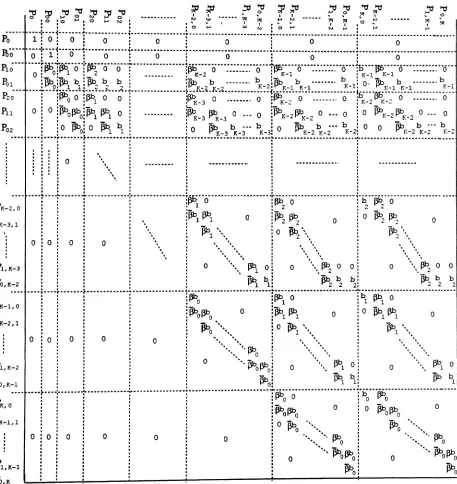
From the above equations, we obtain the transition probability matrix of the system shown

in Figure 5. Thus, the steady state probability, Pi,j, can be computed using a numerical

a

a

... J3bo

... Ph

o

J3b

o

Pb

o o o o o o o o o , ,,_, , o o o o o o o o o o o o

~ ~

:;J

~

:J' ::P

J1

?!

r

;sJ.~

'f

f!

"

:;0

~:;'~

:F

.:0

o :0 : 0 ~: 0 ~ '" : • t: ~ ~ ~ ~ • t"' i: ~ ~ •0 t"' ~ ~ " . • • 0 . . . . , W '" • 0 ...., " ' . . . . , . . . , ....

- . . -:.- .. i - . - -- ..~.- . - . - . - - - - . -~- . - - - -. --.. -..~- -. -- - -- -- - . - _. __ . :. _ _. _ __ .. : . _.. . _. _. _.. _

1 : 0 : 0 : 0 : 0 : 0 : 0 : a

....: i-···~··· ~ _..~ - ~ _ _ : _ _ _

0 : 1: 0 : 0 : 0 : 0 : a : a

••••~Ah-:-ti,;····.:-l'.a~•••••.... .:.••.•..•....•...•~••...•...•••••.•••••.••':'a~···.It_·· ••l:fl=\••••••••••••••••••••••

:..,-, :"'-1 a •~ 0 a : :~ a 0 :1-""': 0 0 :0 I-""': 0 0

o :_ 0:_ : _ 2 : • .... :_ K-2 :_ K-I : K-I_ K-I

:Ah :Ah b •Ah b b : .Ah b u _ _ b .Ah b · b : o. Ah b b

• ,.,....0.,.,....1 1:,.,....~ 2 ? ''''-K'-? K'_? K-2. """'K-I K-l x-.i: ..,....F~-I K-l K-l

...T·"1i3b

₀

"O·

:~I···O···~"·

r···..··..

···r~~~3·~· ;.~.:::::::

...

~. ··1~K··:··O···

..:.:.:..

0·"

!bK·~ ·2·~~·"'···0···::::::::·

0···

. . : • , K- • -.... • ...

• 0 ' A h ' - • '- .- , Ah

0:

pJ....

o(3bo:J3b1 J3b1 0 ~ ~~-3 ~-3 0 ... 0 ~J3bK-2 ~-2 0 ... 0 ~ 0 V'""K-2 J3b_{K- 2} 0... a

: : 0 Ah: 0 ~ b : : Ah b · · · b : 0 Ah b · · · b : 0 0

'Ph

b · · · b

: : """'0: 1 1 : :0 tJ"""K-3 K-3 K-3: fJ"""K-2 K-2 K-2: K-2 K-2 f~-~

····I····r····.··~

..·· ·

"

_ _

: : :

: :

:

:

: : :

: :

:

:

: : 0 : ' , : : : :

: :

:

' : :

:

:

: : :

: :

:

:

' "

' .

.

.

~ :..---.. .:. --- u: -- -

!pli'.

i;

_u.--.. --.---'.t~·

·0"·----

----

~.b --j3i:i' -

-0- --

---.,.,

• 1 • 2 2 2

:i3b

1I3bI 0 1;3b2

~

0 0 ;3b2

~

PhI '

0 ;3b., \

~2

• •

.

'" ',

...

.

Aha a \~OO 0 \~OO

"""'1 " 2 \ 2

PhI

bl , ';3b2

~ ~.

i3b

2

~ ~

.... ····r···~··· -:- .

~J3b0 ~f3b1 0 • b1 13b1 0

';3b0131'0 0 ~PhlJ3b₁ 0 0 ~lJ3b₁

,

.

i3b

o """

~0

PhI '

Ph

1

-.

: , "

... ' ' ' ' ' o A h : ..

... """"0 : \

... Ph

_oJ3b

0~ 0 J3b1 0

Pho~ phI b1 :

.

.

...~ ···T~··o··· ·b~···I3b~···_····

,Ph

ol3bo 0 0

i3b

ol3bo 0

o

i3b

_o .... ;3bo

... ... ..., Po a~·" PI;·" POI P20

PI I

P

0 2

P1 , K- 3

PO, K- 2 PK-I,O

*P=l-P

3.2

The Waiting Time Distribution of the High Priority Cell

Let Xo be the time interval between the arrival instant and the beginning of the next slot,

and let w be the waiting time in the system. We have

w=

Xo

1

+

Xo

2

+

~o

3

+

Xo

K - 1

+

Xo

, l-~K.O

[Po

+

Po,o(l -

u)]

[

K( l )

K-l(l) .

]

'l-~K.O

.r;

0 PO,ju(1 - u)

+.r;

1 PIji - u)(l - u)

[

K -IK -i ( K _ 1 ) . ]

'l-~K.O

?=?=

i pi,jUK-1-'(1 -

u)i(l -

u)

t=O 1=0

The distribution of the waiting time is as follows:

l-~K.O

[Po

+

Po,o(l -

u)] ,

n

=

O.

P[w

=

n

+

Xo]

=

The mean waiting time of a high priority cell can be obtained by the following

argument. Let Pi~ be the probability that an arriving high priority cell finds the system in

state (i,j) given that the high priority cell will be accepted into the system and let NQh be

the average number of high priority cells in front of the arriving high priority cell. We get

NQ h

==

K-l K-i

~_{L..J L..J}' " ipfl._"',3

i=O j=O

1 K-l K-i

1-

P

L L

iPi,j

K,O i=O j=O

The residual service time ltV_o seen by the arriving high priority cell is found as follows:

W

o

==

1

[xoPo

+

(1 -

Po - PK,O)

f(xo

+

i)(l _

(j)(ji]

1 - PK,O i=O

1 [xo(l _

PK,O)

+

(_0'_)

(1 -

Po - PK,o)]

1 - PK,o 1 - 0'

Thus, WH, the mean waiting time of tile high priority cell is :

1

4

Computation of the probability that a low priority

cell will get served and mean waiting time.

In this section, we obtain exact results for the low priority cells. In particular, we calculate the probability that a low priority cell will get served given that it entered the queue. We also obtain the mean waiting time of a low priority cell given that it entered the queue and it got served. The main vehicle for obtaining these results is the one dimensional random walk consisting of the absorbing states 0 and K+l, as shown in Figure 6.

o

1

2

3

K-1

K

K+1

mJ :

Good absorbing state ( cell gets service).

ttl :

Bad absorbing state (cell gets pushed out of queue).

Figure 6: The states of the random walk.

TIle states of the ra.ndom walk are defined as follow. We tag a low priority cell

when it enters the queue. The state variable of the random walk indicates the position of this tagged cell throughout its residency in the queue immediately after a high priority cell arrives. We note that the positions in the queue are numbered from 1 to K. The position

in front of the server is numbered

o.

The tagged unit receives service if the random walk

reaches the absorbing state 0, and it is pushed-out if the random walk reaches the absorbing

state

K+l.

If upon arrival the tagged unit sees i high priority cells and j low priority cells

4.1

Computation of the transit ion probabilities

Let Pi--+_j be the transition probability from state i to state j. Let S, be the probability of

having i cells served during the interarrival time of the high priority cell. Let P[ta

==

n]

be

the probability that the interarrival time of the high priority cell is n slots and 1 - a be the

probability of having a service completion in one slot. Then, for j

>

0, we have

Pi--+_i

P[(i -

j

+

1)service completions]

Si-i+1

f (

i _

~

+

1 ) (1 - u)i-i+1un-(i-i+1)P[ta

==

n]

n=O J

( 1 )i-i+l 00 ,

- (j

L

n.

(jn-(i-i+l)P[t =

n]

(i-j+l)!

n=i-i+l

(n-(i-i+l))!

a

(1 -

(j )i-i+l T(i-i+1 ) ((j)

(i-j+l)! a

and, for j

==

0, we have

i-I

Pi-+O

==

1 -

L

Si i=O

where

TJi-i+

1 ) is the

(i

+

j - 1

)th

derivative of

Ta(z)

at

z

==

a ,and

00

Ta(z)

==

L

znp[ta

==

n].

n=l

The above generating function is computed as follows. Let ta be ~he t.ime interval from. an

active state to an arrival of the high priority cell and ti be the time interval from an Idle

state to an arrival of the high priority cell. We have

{

1

+

1

t

a ,po.(3,p(l - 0.(3)

1

+

ti ,1-P

{

1

+

1ti , (1 -,q q)a(3

1

+

ta ,(1 - q)(l - 0.(3)

Hence,

We get

Ta(z)

za,B[p

+

z(l -

p - q)]

(1 -

a,B)(p

+

q -

1)z2 -

[q

+

p(l -

a,B)]z

+

1

4.2

TIle probability that a low priority cell will get served

Let U,be the probability that the random walk system reaches the absorbing state 0 given

that the system starts in state i. Let Sj be the probability of having j cells served ill an

interarrival time of the high priority cell. We have

Uo=landUK+1=O.

To find

Ui,

i

=

1,2,· . ·,K, we have to solve the following linear equations :

U

1

SoU

2

+

(1 -

So)Uo

1

U

2

SoU

3

+

SlU2

+

(1 -

L

SI)UO

1=0

K-2

U

K -1

SoU

K

+

SlU

K -1

+ ... +

SK-2

U

2

+

(1 -

L

Sl)U

O l=O

K-l

UK SOUK+1

+

SlUK

+ ... +

SK-1U2

+

(1 -

L

SI)UO

. l=O

Thus, we get:

o

+

K-l

(1-

L

SI)UO

[=0

The above system of linear equation is solved numerically ill order to obtain U₂,U₃, · · · ,UK.

Using

U

2 and

U

owe can also calculate

U

1 • Thus, P6~r1Jice'the probability that a low priority

cell will receive service given that it entered the queue is:

K-IK-l-·i

Po

+

L L

Pi,jUi

+

j+1 i=O j=O

K-IK-l-i

Po+ ~

c: c:

~ p .._'1.,3

i=O j=O

-4.3

Mean waiting time of a low priority cell

Let P

o(n,

i)

be the probability that the random walk system reaches absorbing state 0 after

exactly n high priority arrivals given that it sta~ts in state i. We have

Po(O,

i)

i-I

1-

LSi

;=0

i+1

Po(n,

i)

L

Po(n - 1,j)Si+l-i

;=2

K

Po(n, K)

=

L

Po(n -

1,j)SK+l-j

j=2

for n

2:

1and 1

S

i

< [{

Let

N

o(

i)

be the expected number of high priority cells that arrived before the system reached

absorbing state 0 given that the system starts in state i. We get

for i

==

1,2,···,K -1,

00

No{i) =

L

nPo(n, i)

n=O i+1 00

L L

nPo(n -

1,j)Si+I-; j=2n=1

f.

Si+l-i

{~(n

- l)Po{n - 1,j)

+

~

Po{n - 1,j)}

i+l 00 i+l 00

L

Si+l-j

L

nPo(n,j)

+

L

Si+l-j

L

Po(n,j)

j=2 n=O j=2 n=O

i+l i+l

L

Si+l-j

N

o

(j )

+

L

Si+l-j

U

j

;=2

;=2

and

00

No(K)

=

L

nPO(n,

K)

n=O

K 00

L L

nPO(n - 1,j)SK+I-;

j=2n=l

t.

SK+l-i

{~(n

- l)Po{n - 1,j)

+

~

PO{n - 1,j) }

K o o K 00

:E

SK+l-i

:E

nPO(n,j)

+

~

SK+l-i

:E

PO{n,j)

K K

·L

SK+l-jNo(j)

+

L

SK+l-jUj

;=2

;=2

To find N_o(

i), i

== 1,2,· · · ,K, we solve the following linear equations numerically:

No(l)

N

o(2)

3

SlNo(2)

+

SoNo(3)

+

L

S3-

j

U

j

j=2

K

No(K -

1)

SK-2

N

O(2)

+

SK-3

N

O(3)

+ ... +

SoNo(K)

+

L

SK-jU

j

j=2 K

No(K)

=

SK-

1N

o

(2)

+

SK-2 NO(3)

+ ... +

SlNo(K)

+

L

SK+l-

jU

j

j=2

Thus, N_o(i), the expected number of high priority cells that arrive before the tagged low

priority cell gets served given that the tagged low priority cell will get served, is:

TIle mean waiting time of the low priority cell given that it gets served, WL , is:

K-l

K - l - i

Po

+

L L

P

i,jUi+j+l

5

Approximate analysis of the switch

In this section, we describe a simple approximation algorithm for the analysis of the ATM

switch. The approximation algorithm utilizes expression( 3) for a , and the exact results

obtained in sections 3 and 4. The algorithm is an iterative scheme. III each iteration we

need the cell loss probability for each packet processor queue irrespective of the priority of the lost cell. For efficiency purposes, we calculate this cell loss probability using an algorithm

for analyzing a single-class IBP /Geo/l/K+l queue that was presented in [27].

The iterative approximation algorithm involves the following steps:

step

o.

Set initial value of the utilization of the ith cell processor, p~O),i := 1,2· ..N.

step 1. Compute the probability of retransmission of a cell due to contention ill the Clos

ATM switch, 00(0),using expression 3.

step 2. Solve the

IBP/Geo/1/K

+ 1 queue with a single class of cells using the solution

method in [27] in order to find the probability of cell loss due to the fact that the buffer

is full, IK.

step 3. Compute the utilization of the cell processor, pP) :

pP)

=

a(I -

q) (I-,K)

2-p-q ,i=1,2.··N.

step 4. Use expression 3 to compute u(1) the probability of retransmission of a cell due to

contention in the Clos ATM switch with the new cell processor utilization,

p~l),

i

=

1,···,N.

step 5. Iflu(l) - u(O)1

<

e then o

=

u(1) and go to step 6, else set u(O) = u(1) and go to step

2.

step 6. Solve the two-class I

BP/Geo/I/

K

+

1queue with head-of-line with no preemption

and push-out to find the blocking probability of the high priority cell, PK,O'

step 7. Compute the probability that a low priority cell gets served and its mean waiting

6

Numerical Results

TIle approximation algorithm described in the previous section was employed to analyze a

16 X 16 bufferless Clos ATM switch. Each switching element was a 4 X 4 crossbar switch.

The system size of each cell processor queue was set equal to 32. The arrival process to

each cell processor was assumed to be an IBP with a == 1. That is, during the busy period

each slot contains a cell. The approximation results were compared against results obtained by simulation. TIle results are summarized in figures 7 to 19. Figures 7 to 11 are for a symmetric case, and figures 12 to 19 are for two different asymmetric cases.

In the symmetric case, we assume the same arrival process to each input link with an average arrival rate 0.3. Each arriving cell chooses one of the destination output links uniformly. In figures 7 and 8, we plot the approximate and simulation results for the mean

waiting time for high respectively low priority cells as a function of (3 for various 02 _values.

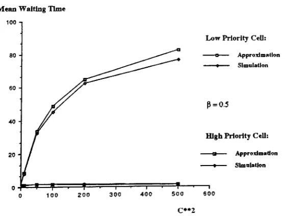
In figure 9, we plot the approximate and simulation results for the probability that a low

priority cell gets served given that it entered the queue as a function of (3 for various C2

values. The approximate and simulation results for tile cell loss probability for low priority

cells is given in figure 10 as a function of C2 _{for (3 equal to 0.3. We note that the cell loss}

probability of the low priority cells comprises the probability a low priority cell will arrive

to a full queue and the push-out probability. In Figure 11, we plot the approximate and

simulation results for mea.n waiting time for high and low priority cells as a function of C2

for (3 equal to 0.5.

In the results given in figures 7 to 10, the minimum relative error was 1

%,

the

maximum relative error was 15%, and the average relative error was 7%. Most of the

approximate results had a relative error less than 5%. The curves given in figures 7 and

8 show how the mean waiting time is affected by 02 _{and {3. When C}2 _{is high (i.e. bursty}

arrivals), the mean waiting time of the low priority cells drops when f3

==

0.9. This is due

to the fact that most of the low priority cells are pushed-out of the buffer by high priority

cells. Figure 9 shows how the probability that a low priority cell gets served is affected by

the value of

C

2

and (3. In particular, we note that this probability significantly drops as

C

2

Increases.

In the two asymmetric cases considered here, the following assumptions were rnade regarding the arrival processes.

case 1:

Ai

== 0.4,i == 1,2,···,8 with

C2

== 100,

Ai

==

0.1,i == 9,10, · · · ,16 with C2

==

_10.

case 2:

Al

== 0.4, Al6 == 0.1 , and the values of the remaining

Ai'S

were linearly distributed

between 0.4 and 0.1. TIle value of

0

2

was the same for all 16 arrival processes and it

Mean Waiting Time of tbe High Priority CeU

20

- - - C··2dO, Appro:dms.tlon

- - 0 - - C··2=50, Simulation

- - - - C...2=10, Approximation - - . - - C**2=10, SlnmJation - - - - 0·2=100, Approximation - - - . - - <:-"'1=100, Simulation

1.0 0.8

0.6 0.4

0.2

5

- m - - <:**2=1,Approximation - + - - <:*·2=1. Simulation

O-t-""'T""""'"'~--r---r----,-~--r--r---r---"--,.--,,...--,r--_

0.0 10

15

Figure 7: Mean waiting time of the high priority cell; symmetric case.

In both asymmetric cases, it was assumed that each arriving cell chooses one of the destina-tion output lines uniformly.

Figures 12 to 14 are for the asymmetric case 1, and the remaining figures a.re

for the asymmetric case 2. In all the figures we give approximate and simulation results for the most utilized input queue and the least utilized input queue. The relative error of the approximate results is similar to the one observed in the symmetric case discussed above. Finally, we note that the behavior of the performance curves given in these figures is similar to the one observed in the symmetric case.

7

Conclusion

In this paper we presented a queueing model of a blocking bufferless synchronous Clos

ATM switch with input buffers. The arrival process to each input port was assumed to

Mean Waiting Time of theLowPriority Cell

100 80 60 40 20

•

•

•

- - A - C.·2=IOO, ApproxlrTUltion - . . . . - C"Z=lOO,Slmulatl~n

_____ C••Z=50, ApproxJmation

- - 0 - - C··Z=50, Simulation

- - a - - C••Z=10, Approximation

~ C.·2=10, Simulation _ _ _ _ e*·1=1, Approdmatlon - - . - - C ••Z=l, Simulation 1.0 0.8 0.6 0.4 0.2 o-l--.-JII::::;:~==;:::::II:=;=~~:R:;==tIl=::;::::II~=*:::;:a..,--., 0.0

Figure 8: Mean waiting time of the low priority cell; symmetric case.

~ C"=l,Apprmtmatlon

--...-

C··Z=l, Simulation

----

C··Z=10, Approxfmntlon

- . - - C··Z=10, Simulation

----

C··Z=-<G, Approximation

- 0 - - C··Z=50, Simulation

--.-- e*·Z=l00, Approximation

- - - - 6 - - e*·Z=100, Simulation

- - I t - ' C**Z=ZOO,Appro~matlon

---+-- C··Z::200, Simulation 0.8 1.0 P 0.6 0.4 0.2 1.0 0.8 0.6 0.4 0.2-+---T-r--r----,r---r-~-or__r_...,.-.,.___r_-.,..___r____r~ 0.0

Probability that a low priority cell gets served

CellLossProbabUltyfor LowPrIority Cells

10 0

- - m - - Approximation - . . - Simulation

600 400

300 200 100

10 -5-t---r---~....,.--r---'r----r----­

o

Figure 10: Cell loss probability for low priority cells; symmetric case, (3

==

0.3.

Mean Waiting TIme

100

Low Priority Cell:

~ ApproximAtion

~ Simulation

p=o.5

High Priority Cell:

_____ Approximation

--+-- Simulation 600

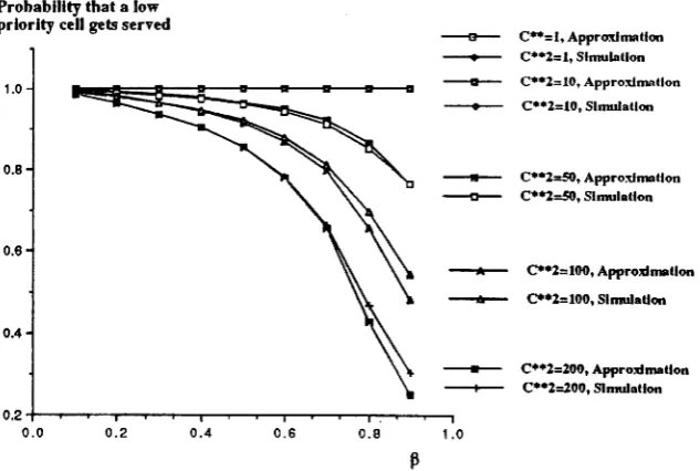
ProbabWtythat alow priority cell gets served

LowUtlllzatlODInput Queue:

1.0 - + - - Slmal8tlon

- - a - - Approximation

0.8

0.6

Hlgh Utillzatlon Input Queue:

- + - - Simulation

- ' I t - - Approximation

0.4

1.0 0.8

0.6

0.4

0.2

0.2-J- -~--r---y-___r-r___r__~___r___,r__~~__,

0.0

Figure 12: Probability that a low priority cell gets served; asymmetric case 1.

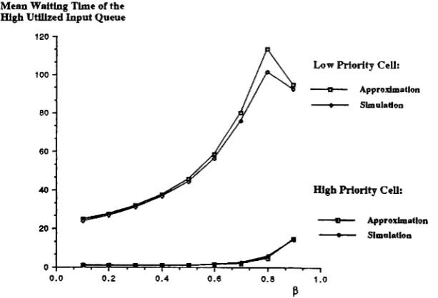
MeaD Waiting Time of the HIgh UtillzedInput Queue

120

- - - Approximation - . . . - Simalation

HIghPrIority CeO: LowPriority Cell:

1.0

- a - - Approximation

- + - - Simulation

0.8 0.6

0.4

0.2

o.+-_a::;::::::::tI~::;:::II~=*==;:=-=;::=*=:::;:~- _

0.0

60

20

40

80 100

Mean Waiting Time of the

LowUtilized Input Queue

6 _{Low Priority Cell:}

5

4

- - - - . - Simulation

- - a - Approximation

3

2

HIgh Priority Cell:

- . - - SlmulnUon

~ Approximation

1.0 0.8

0.6 0.4

0.2

O+-...,....--....~-..-~-r---.--....

...-....--_..._-....-0.0

Figure 14: Mean waiting time for the low and high priority cells of the low utilized input

queue as a function of{3; asymmetric case 1.

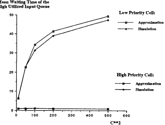
Mean Waiting Time of the Hlgb Utllized Input Queue

120 100 80 60 40

20

Low Priority Cell:

- a - - - Approximation

- - 0 - - Simulation

High Priority Cell:

--m-- Approximation

- + - - Simulation

1.0 0.8

0.6 0.4

0.2

oL.---!R::;::~==;::R::::;:::::~~*=;:=tlIt::::~~----r-~--r---, 0.0

Figure 15: Mean waiting time for the low and high priority cells of the high utilized input

High Priority CeU: Low Priority CeU:

--+-- Approximation

~ Simulation

---D- Approximation - + - - Simulatlqn

20 40 60

Mean Waiting Time of the Low UtUlzed Input Queue

80

1.0

0.8 0.6

0.4

0.2

o-l-~t::;=:=-=:::::;::::I1::;:~:::;::a:;~~~....--....-....--...--..

0.0

Figure 16: Mean waiting time for the low and high priority cells of the low utilized input queue as a function of (3; Asymmetric case 2.

Mean Waiting Time of the High UtUlzedInput Queue

50

40

Low Priority Cell:

- - . - Approximation ---...- Simulation

30

20

10

HIgh Priority Cell:

- - - Approximation

- - + - - Simulation

600

500 400

300 200 100

o~::::$:~~:;::::~==;:=:;::=::::;::::=;:=;::=:::e-_ _

o

Figure 17: Mean waiting time for the low and high priority cells of the high utilized input

Mean Waiting Time of the Low Utilized Input Queue

50

Low Priority Cell:

- - . . . - Simulation

- ' I t - Approximation

High Priority Cell:

- - . . . - SImulation

~ Appromn.tton

Figure 18: Mean waiting time for the low and high priority cells of the low utilized input

queue as a function of 0 2 _{with {3}

=

_{0.3; Asymmetric case 2.}

Cell Loss Probability of theLow Priority Cell

10 0

600

500

C··2

400

- i i i ' - Approximation

- - + - - SImulation

300

Low Utillzed Input Queue:

- - 0 - - ApproxJm.tlon ---.--- 51ma.etlon

High Utilized Input Queue:

200 100

10·6+-J..L...,.-..,---r--r----r--r-__,._-~--,.--.._--r-___,

o

a good accuracy. Using the analytic techniques developed in this paper, various in teresting

performance measures such as cell loss probability, mean waiting time, probability that a

low priority cell gets served, were obtained.

References

[1] J.S. Turner "Design of a broadcast packet switching network ", IEEE Trans. Comrn.,

COM-36 (1988) 734-743.

[2] MJ. Narasimha "The Batcher-banyan self-routing network: university and

simplifica-tion", IEEE Trans. Cornm., COM-36 (1988) 1175-1178.

[3]

A.Huang and S. Knauer "Starlite: a wideband digital switch", Proc. IEEE GLOBECOM

'84 (1984) 121-125.

[4] J. Giacopelli, M. Littlewood, and W.D. Sincoskie "Sunshine: a high performance

sel]-routing broadband packet switch architecture", Proc. Int. Switch Syrnp. '90.

[5] F.A. Tobagi and

T.

Kwok "Fast packet switch architectures and the tandem Banyan

switching fabric", Proc. NATO Advanced Workshop on Architecture and Perfor-mance Issues of High-Capacity Local and Metropolitan Area Networks, June 25-27,1990, Sophia-Antipolis, France.

[6] S. Nojima, E. Tsutsui, II. Fukuda and M.Hashimoto "Integrated services packet network

using bus matrix switch", IEEE

J.

SAC, SAC-5 (1987) 1284-1292.

[7]

Y.-S.

Yeh,

M.

Hluchyj, and A. Acampora" The knockout switch: a simple, modular

architecture for high performance packet switching ", IEEE J. SAC, SAC-5 (1987) 1274-1283.

[8J H. Ahmadi, W.E. Denzel, C. A. Murphy, and E. Port "A high performance switch fabric

for integrated circuit and packet switching", Proc. INFOCOM '88 (1988) 9-18.

[9] M. Devault, J.Y. Cochennec, and M. Servel "The 'Prelude' ATD experiment:

assess-ments and future projects",

IEEE J. SAC, SAC-6

(1988),1528-1537.1528-1537,1988.

[10] H. Kuwahara, N. Endo, M. Ogino, T. Kozaki "A shared buffer memory switch for an

ATil1 exchange", Proc. Int. Conf, Comm. (1989) 4.4.1-4.4.5.

[11]

H.

Suzuki,

II.

Nagano, and

T.

Suzuki "Output-buffer switch architecture for

aSY1t-chronous transfer mode", Proc. Int. Conf. Comm. (1989) 4.1.1-4.1.5.

[12)

F.A.

Tobagi "Fast packet switch architectures for broadband integrated services

[13] M.J. Karol, M.G. Hluchyj and S.P. Morgan "Input us. output queueing on a

space-division packet switch", IEEE Trans. Comm., COM-35 (1987) 1347-1356.

[14] M.G. Hluchyj and M.J. Karol "Queueing in high-performance packet switching", IEEE

J.

SAC, SAC-6, (1988) 1587-1597.

[15] J. H.

Patel"Performance of Processor-Memory Interconnections for Multiprocessors" ,

IEEE Trans. on Comp., COMP-30 (1981) 771-780.

[16]

H.

Yoon,

K. Lee,

and

M.

Liu "Performance analysis of multibuffered packet-switching

networks in multiprocessor sustems";IEEE Trans. Oil Comp., COMP-39 (1990) 319-327.

[17] S.Z. Shaikh, M. Schwartz, and T.R. Szymanski "Analysis, control and design of crossbar

and banyan based broadband packet switches for integrated traffic", IEEE Int, Conf. Comm., VOL. 2 (1990) 761-765.

[18] Y. Oie, T. Suda, M. Masayuki, and H. Miyahara "Survey of the performance of

non-blocking switches with FIFO input buffers", IEEE Int. Conf. Comrn., VOL. 2 (1990) 737-741.

[19] H. Yamashita, H.G. Perros, and S.-W. Hong "An approximate analysis of the shared

buffer switch with bursty arrivals", Proc. NATO Advanced Workshop on Architechure and Performance Issues of High-Capacity Local and Metropolitan Area Networks, JUlIe

25-27,

1990, Sophia-Antipolis, France.

[20]

J.

Garcia and O. Casals, "Priorities in AT!vI networks", Proc. NATO Advanced

Work-shop on Architechure and PerformanceIssues of High-Capacity Local and Metropolitan

Area Networks, June 25-27, 1990, Sophia-Antipolis, France.

[21] J.-Y. Le Boudec "An efficient solution method for Marko» models of ATAl links with

loss priorities", IBM Research Rept.

RZ

2001, 1990.

[22]

H. Kroner, G.

Hebuterne,

P.

Boyer,

A.

Gravey "Priority management in AT!v[ switching nodes", to appear in IEEE Journal on Selected Areas in Communication.

[23] A. Gravey and G. Hebuterne"Mixing time and loss priorities in a single server queue",

Tech. Rept. C.N.E.T, France,

[24] S. Sumita and T. Ozawa "Achievability of performance objectives in AT!vI switching

nodes", Proc. International Seminar on Performance of Distributed and Parallel Sys-terns, Kyoto, Dec. 1988, 45-56.

[25] N. Yin,

S.-Q.

IIi and T .E. Stern"Congestion control for packet voice by selective packet

discarding", IEEE Trans. COIIlm., VOL 38 (1990) 674-683.

[26] H.G. Perros "Performance issues in ATlIfnetworks - A literature review", Tech. Rept.,

[27] A. A. Nilsson, F.- Y. Lai, and H. G. Perros "An Approzitnate Analysis of a Bufferless